In the previous blog post
here I implemented Bézier curves. There are other important structures that are used in computer graphics and I'd need those structures to define a domain and a solution in IGA for my implementation here:
https://github.com/carlonluca/isogeometric-analysis.
Bézier curves are great, but the polynomials needed to describe some curves may need a high degree to satisfy multiple constraints. To overcome this problem, some structures were designed to use piecewise-polynomials instead. Examples in this case are NURBS and B-splines.
B-spline Curves
B-splines are curves that are described using piecewise-polynomials with minimal support. The parametric domain is split into multiple ranges by using a vector. The general definition of a B-spline curve is:
$$\boldsymbol{C}\left(\xi\right)=\sum_{i=0}^{n}N_{i}^{p}\left(\xi\right)\boldsymbol{P}_{i},\;a\leq\xi\leq b$$
where $\boldsymbol{P}_{i}$'s are the control points of the curve and the functions $N_{i}^{p}\left(\xi\right)$ are basis functions defined as:
$$N_{i}^{0}\left(\xi\right)=\left\{ \begin{array}{ll}1, & \xi_{i}\leq\xi<\xi_{i+1}\\0,&\text{otherwise}\end{array}\right.,a\leq\xi\leq b$$
$$N_{i}^{p}\left(\xi\right)=\frac{\xi-\xi_{i}}{\xi_{i+p}-\xi_{i}}\cdot N_{i}^{p-1}\left(\xi\right)+\frac{\xi_{i+p+1}-\xi}{\xi_{i+p+1}-\xi_{i+1}}\cdot N_{i+1}^{p-1}\left(\xi\right),a\leq\xi\leq b$$
The values $\xi_{i}$ are elements of the aforementioned knot vector, defined as:
$$\Xi=\left[\underset{p+1}{\underbrace{a,\ldots,a}},\xi_{p+1},\ldots,\xi_{n},\underset{p+1}{\underbrace{b,\ldots,b}}\right],\left|\Xi\right|=n+p+2$$
where $p$ is the degree of the basis functions. A knot vector in this form is said to be nonperiodic or clamped or open.
B-spline Surfaces
By using the tensor product we can obtain B-splines in spaces of higher dimension. For surfaces, given the knot vectors:
$$\Xi=\left[\underset{p+1}{\underbrace{a_{0},\ldots,a_{0}}},\xi_{p+1},\ldots,\xi_{n},\underset{p+1}{\underbrace{b_{0},\ldots,b_{0}}}\right],\left|\Xi\right|=n+p+2$$
$$H=\left[\underset{q+1}{\underbrace{a_{1},\ldots,a_{1}}},\xi_{q+1},\ldots,\xi_{m},\underset{q+1}{\underbrace{b_{1},\ldots,b_{1}}}\right],\left|H\right|=m+q+2$$
a B-spline surface can be defined as:
$$\boldsymbol{S}\left(\xi,\eta\right)=\sum_{i=0}^{n}\sum_{j=0}^{m}N_{i}^{p}\left(\xi\right)N_{j}^{q}\left(\eta\right)\boldsymbol{P}_{i,j},\;\left\{ \begin{array}{c}
a_{0}\leq\xi\leq b_{0}\\
a_{1}\leq\eta\leq b_{1}
\end{array}\right.$$
where $p$ and $q$ are the degrees of the polynomials.
In the implementations, sometimes I preferred the matrix form of the equations:
$$\boldsymbol{C}\left(\xi\right)=\left[N_{i-p}\left(\xi\right),\ldots,N_{i}\left(\xi\right)\right]\cdot\left[\begin{array}{c}
\boldsymbol{P}_{i-p}\\
\vdots\\
\boldsymbol{P}_{i}
\end{array}\right],\;\xi\in\left[\xi_{i},\xi_{i+1}\right)$$
For the surfaces instead, the matrix form is:
$$\boldsymbol{S}\left(\xi,\eta\right)=\left[N_{i-p}\left(\xi\right),\ldots,N_{i}\left(\xi\right)\right]\cdot\left[\begin{array}{ccc}
\boldsymbol{P}_{j-q,i-p} & \cdots & \boldsymbol{P}_{j-q,i}\\
\vdots & \ddots & \vdots\\
\boldsymbol{P}_{j,i-p} & \cdots & \boldsymbol{P}_{j,i}
\end{array}\right]\cdot\left[\begin{array}{c}
N_{j-q}\left(\eta\right)\\
\vdots\\
N_{j}\left(\eta\right)
\end{array}\right],$$
$$\xi\in\left[\xi_{i},\xi_{i+1}\right),\eta\in\left[\eta_{j},\eta_{j+1}\right)$$
These forms leverage a more performant algorithm for the computation of the basis functions, which returns the value of all nonvanishing functions for a point in the parametric space. The Octave implementation is clearly simpler as Octave has native support for matrices, the TypeScript implementation instead includes a basic
Matrix2 class that offers the simplest operators.
Octave Implementation
An implementation for Octave is provided in
https://github.com/carlonluca/isogeometric-analysis/tree/master/3.4. There are examples to show how to draw B-spline curves with the implementation.
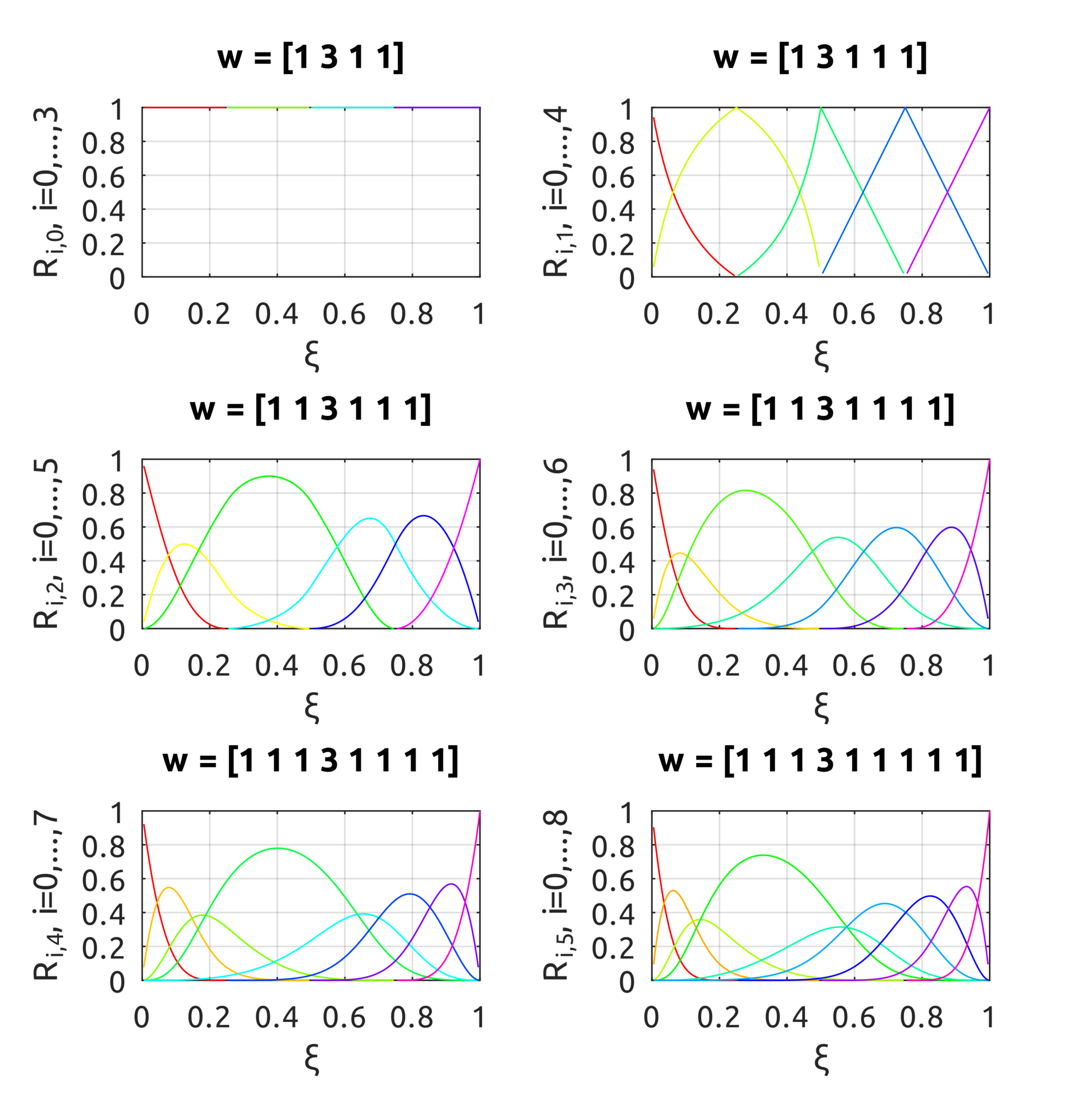
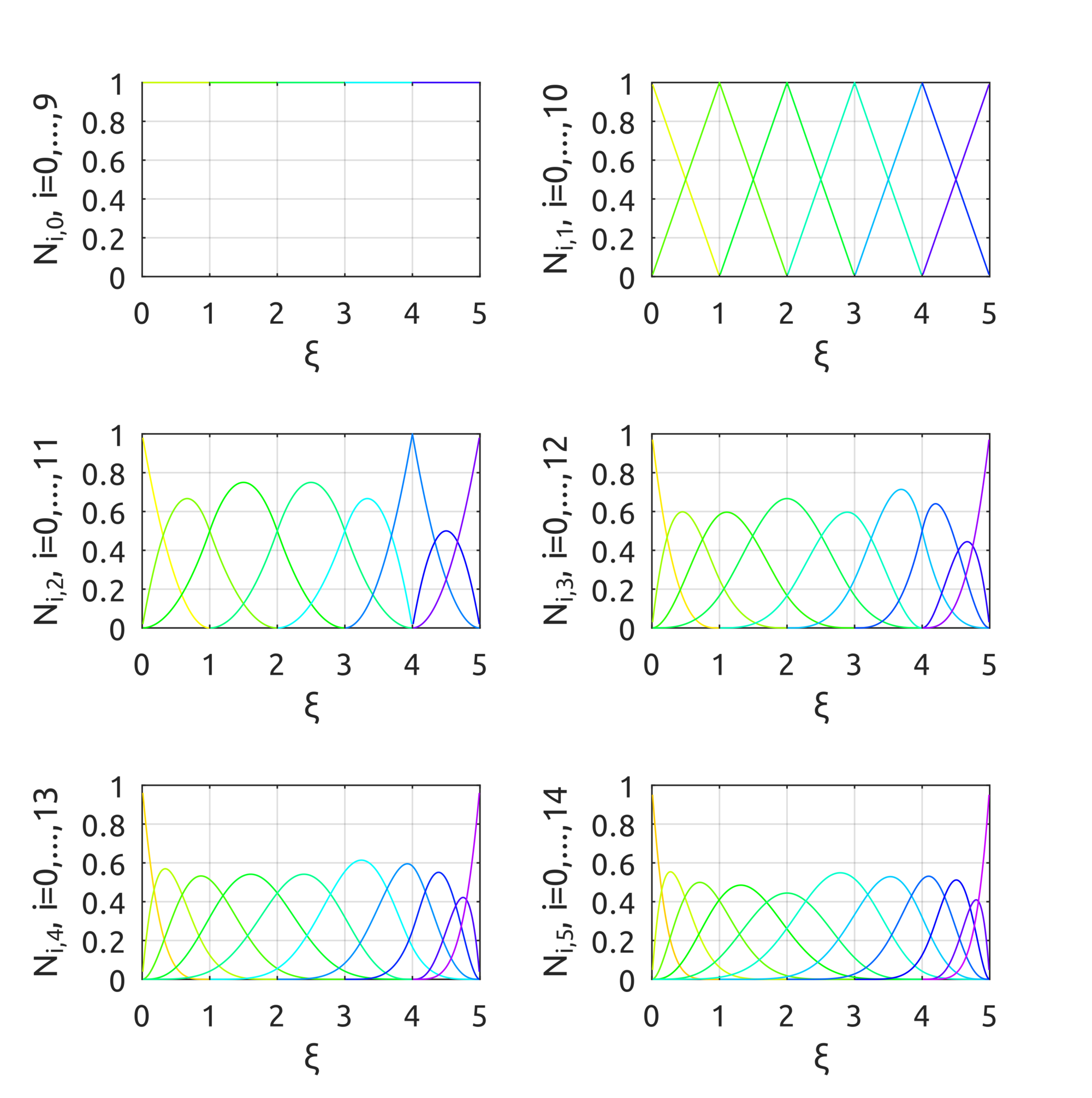
For example, the
drawBsplineBasisFuns script shows the B-spline basis functions over the knot vector $\Xi=[0, 0, 0, 1, 2, 3, 4, 4, 5, 5, 5]$ using the provided implementation of the basis functions:
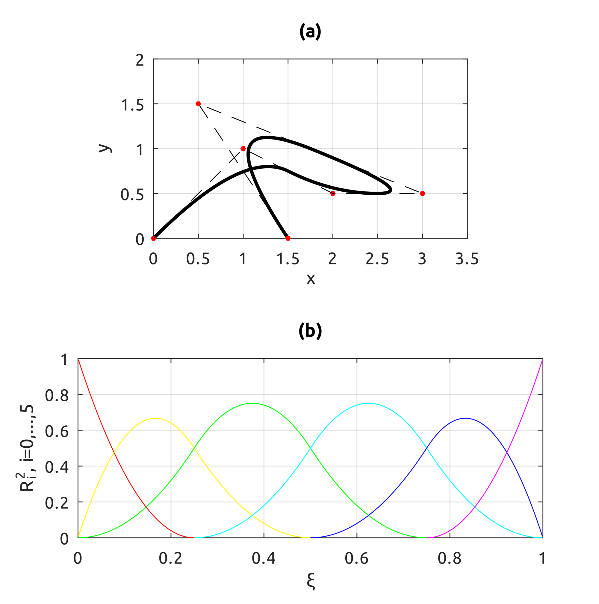
The
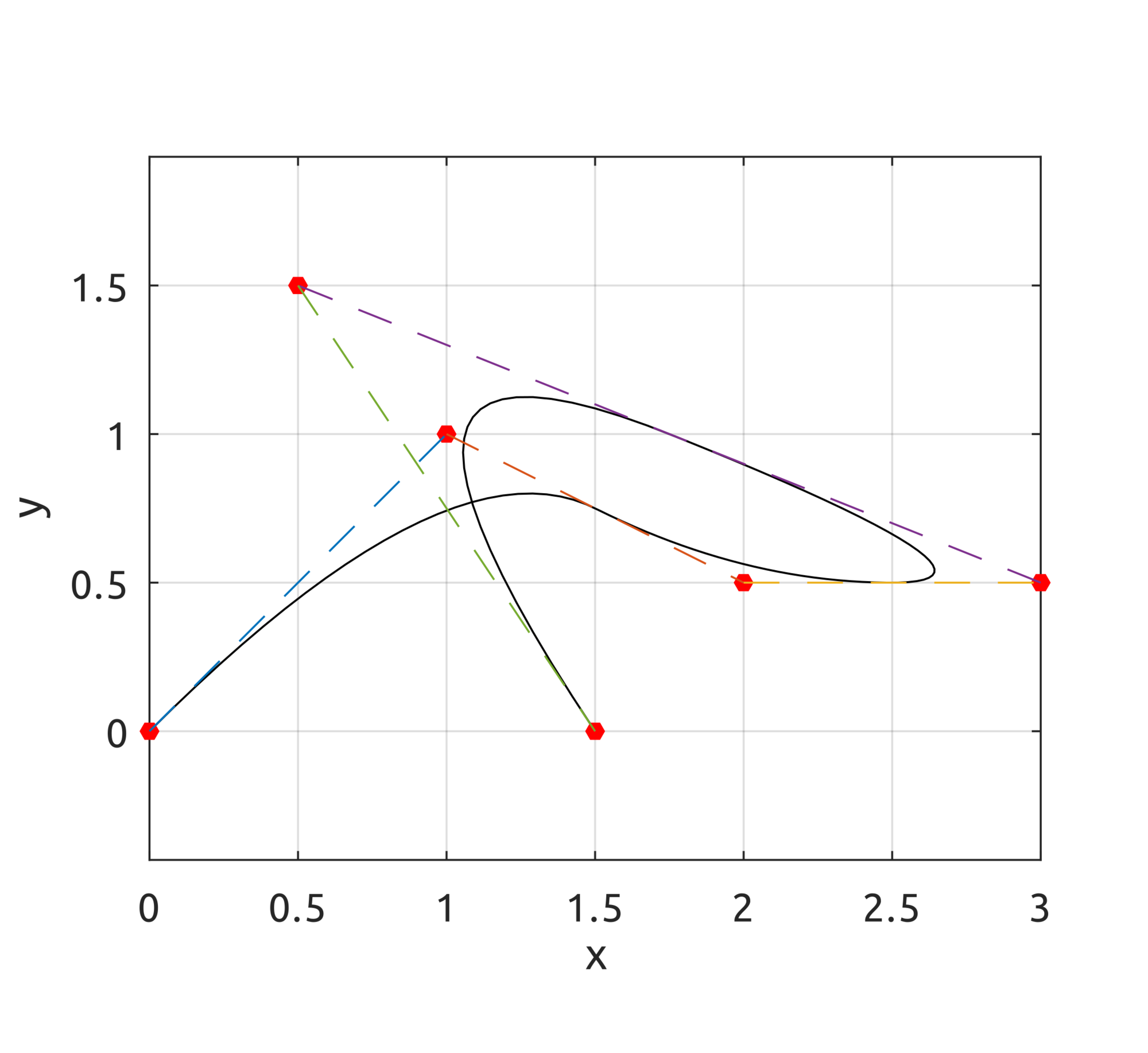
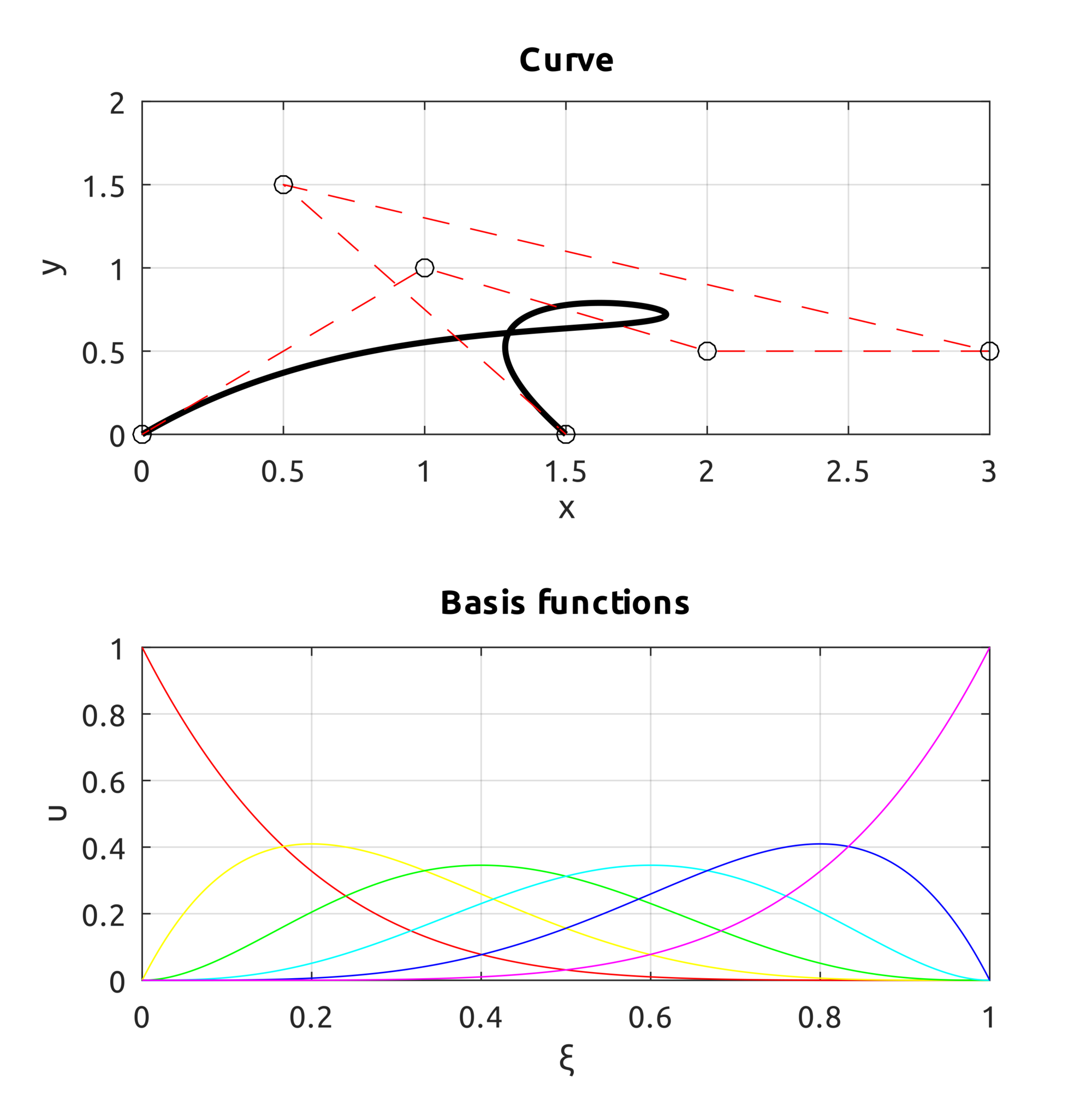
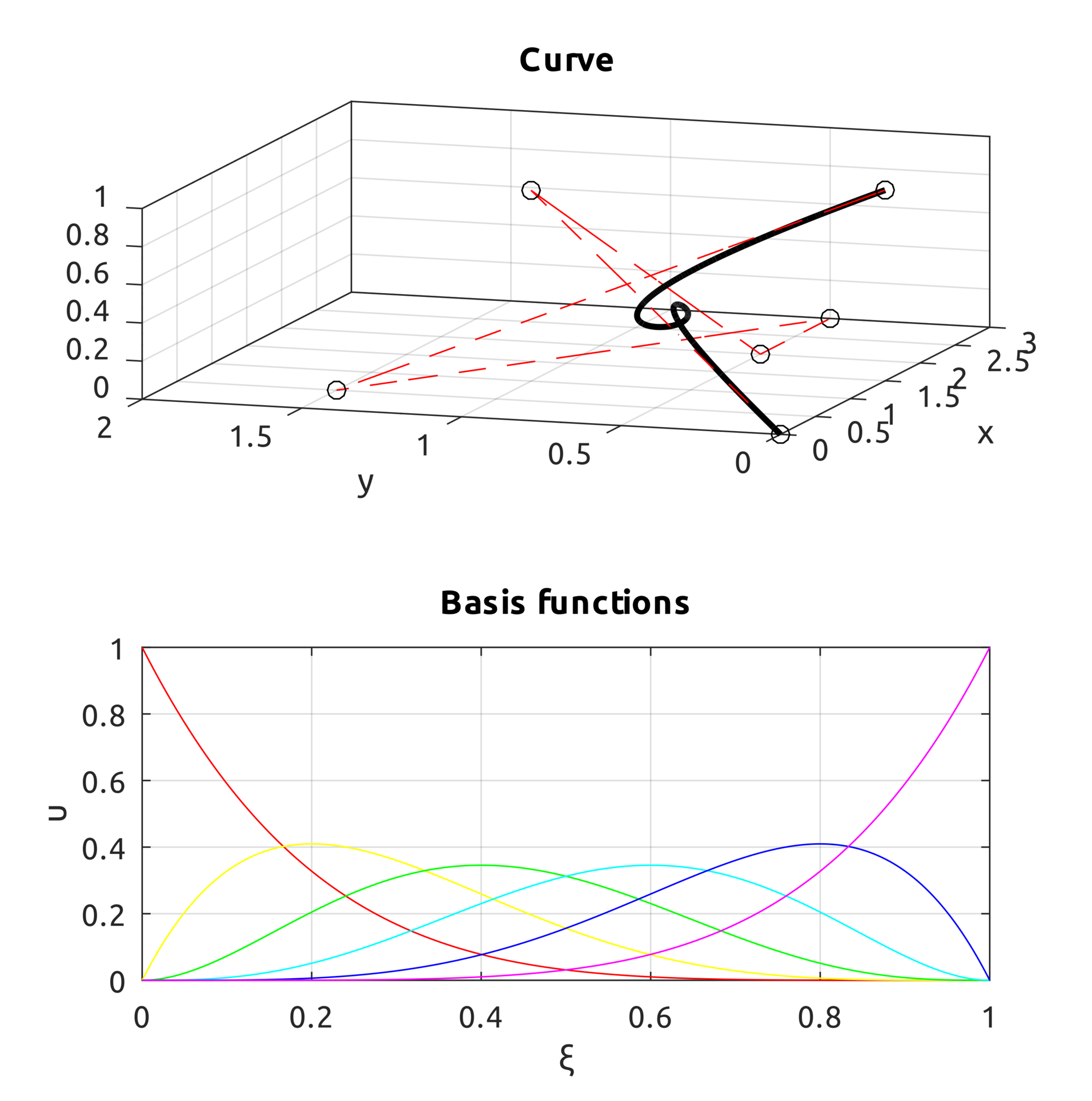
drawBsplineCurve script draws, instead, the real curve. For example, to draw the B-spline of degree $p=2$ defined over the knot vector $\Xi=[0, 0, 0, 0.25, 0.5, 0.75, 1, 1, 1]$ with control points:
$$\boldsymbol{P}_{0}=\left(0,0,0\right),\;\boldsymbol{P}_{1}=\left(1,1,1\right),\;\boldsymbol{P}_{2}=\left(2,0.5,0\right)$$
$$\boldsymbol{P}_{3}=\left(3,0.5,0\right),\;\boldsymbol{P}_{4}=\left(0.5,1.5,0\right),\;\boldsymbol{P}_{5}=\left(1.5,0,1\right)$$
a simple call to:
drawBsplineCurve(5, 2, [
0, 0, 0, 0.25, 0.5, 0.75, 1, 1, 1
], [
0, 0; 1, 1; 2, 0.5; 3, 0.5; 0.5, 1.5; 1.5, 0
]);
draws:
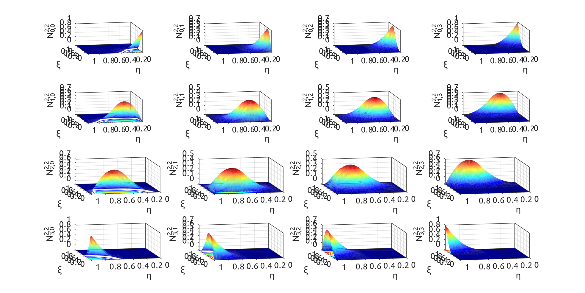
For surfaces,
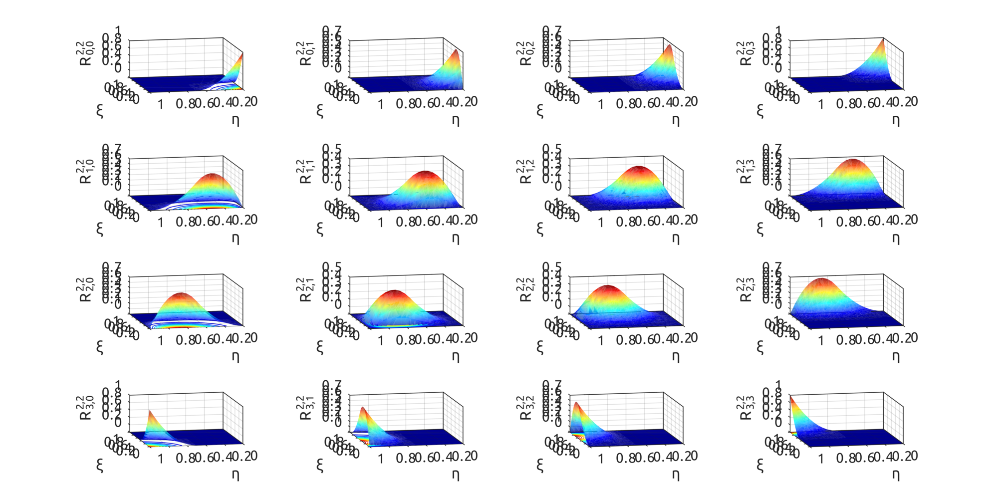
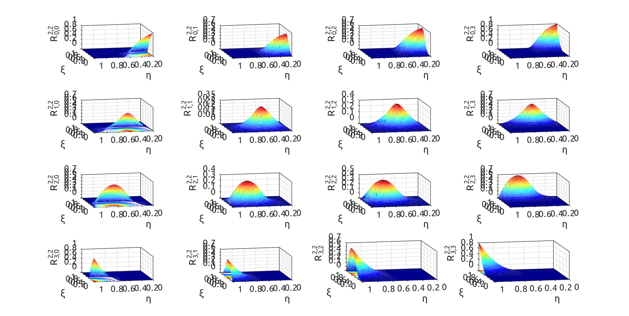
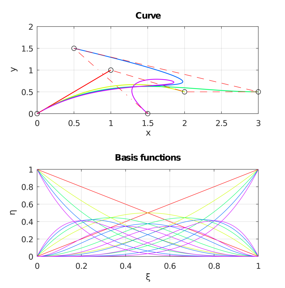
drawBivariateBsplineBasisFuns can be used to draw bivariate basis functions. For example:
drawBivariateBsplineBasisFuns([
0, 0, 0, 0.5, 1, 1, 1
], 3, 2, [
0, 0, 0, 0.5, 1, 1, 1
], 3, 2);
gives this result:
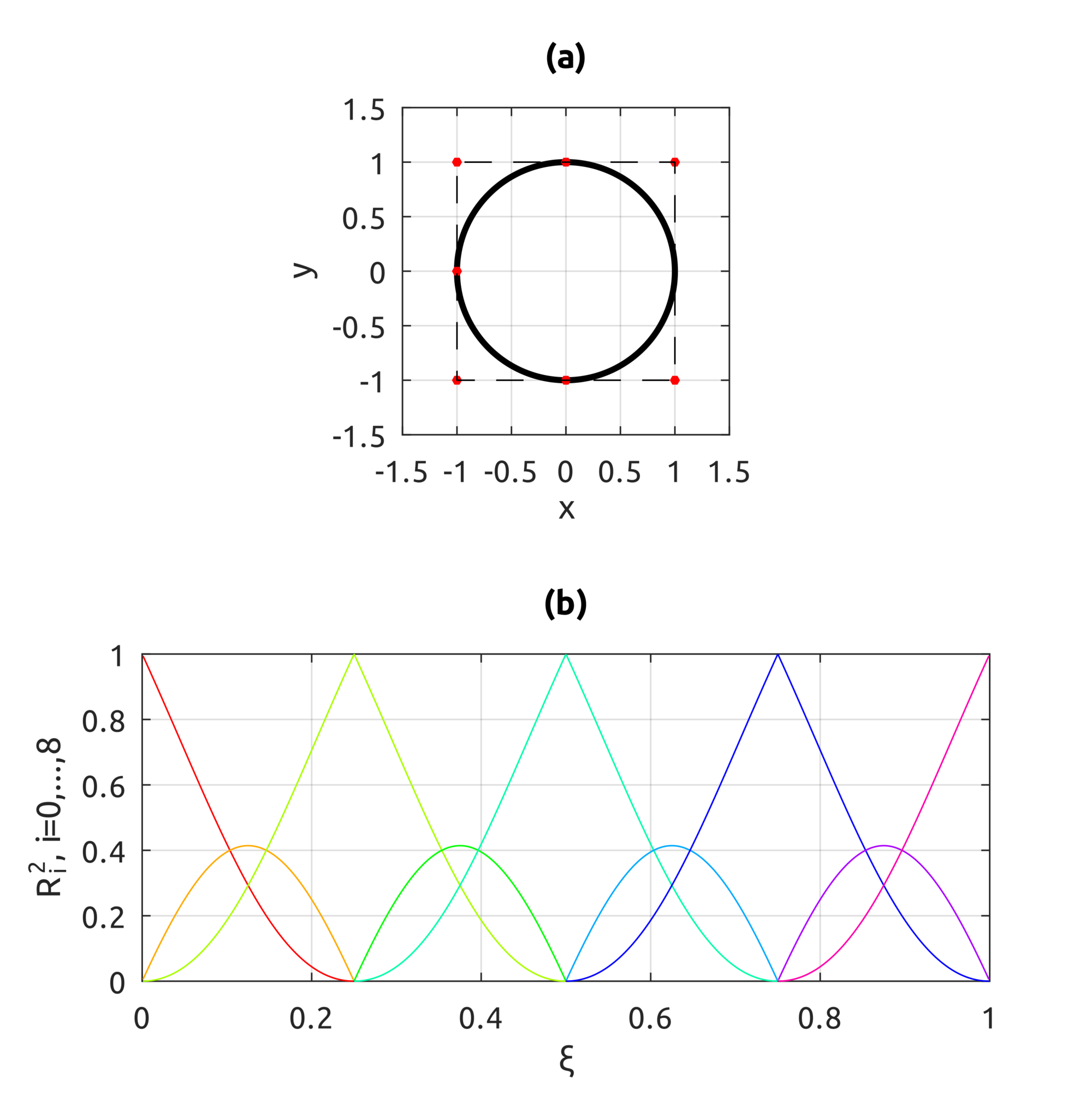
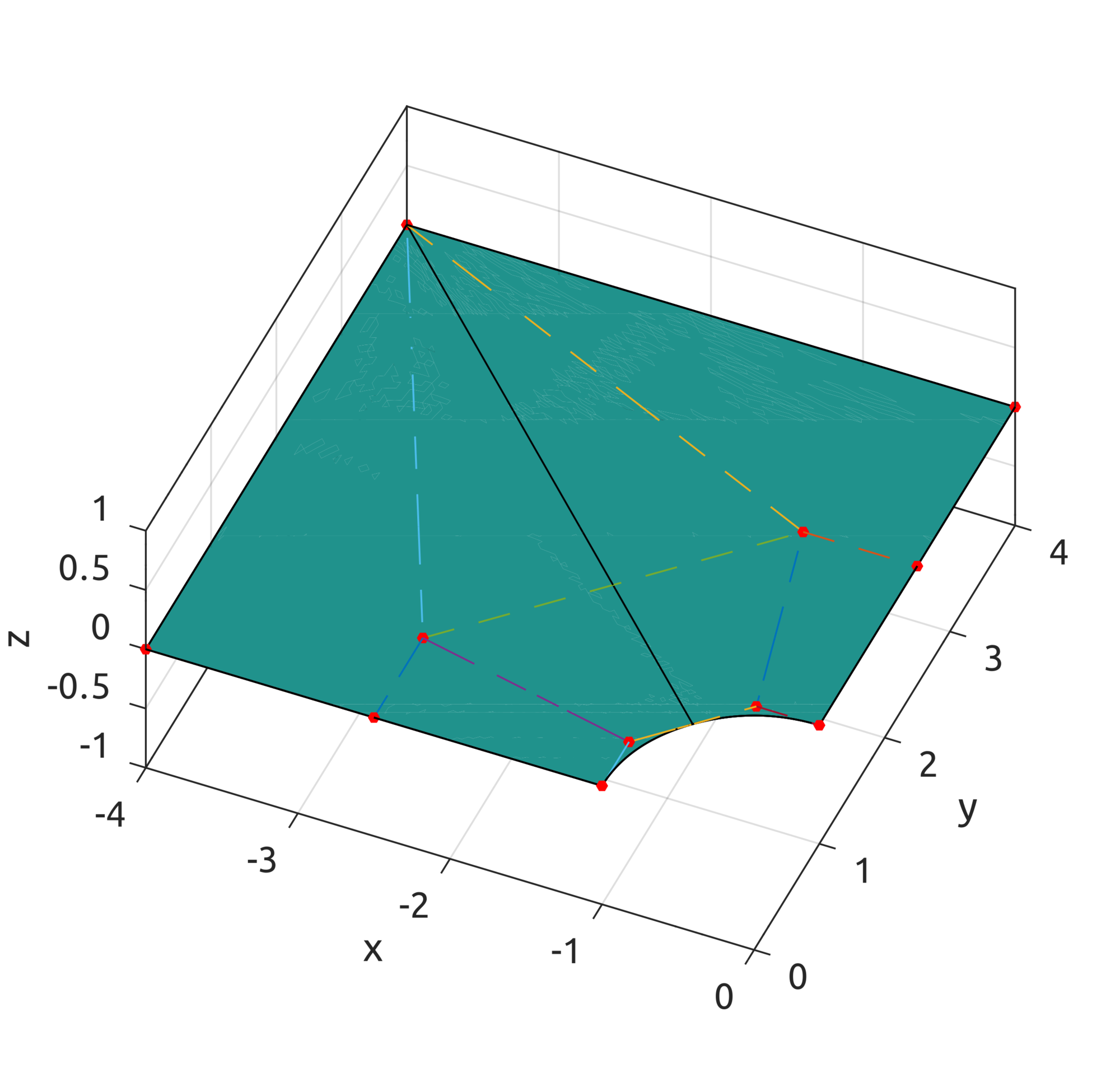
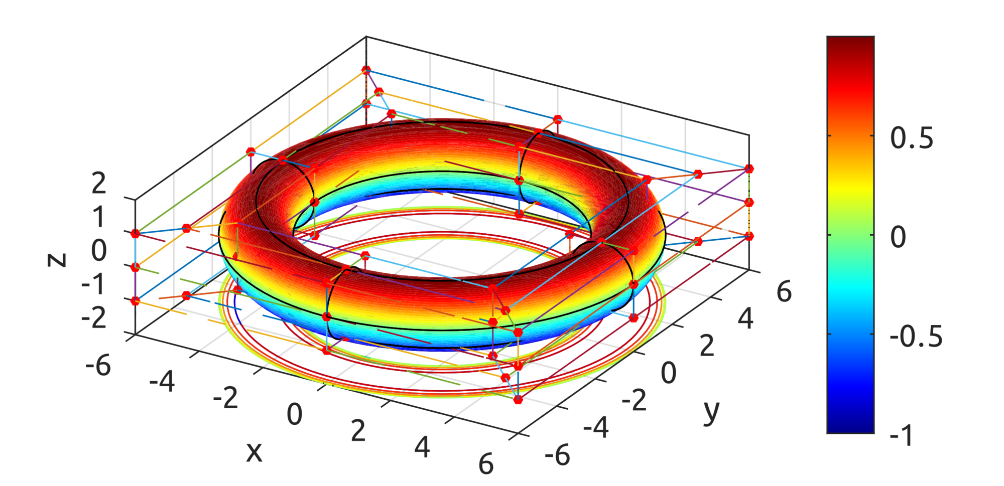
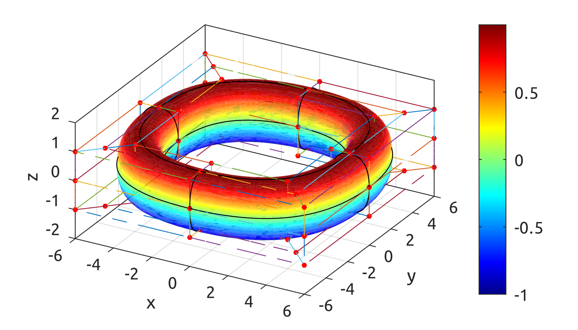
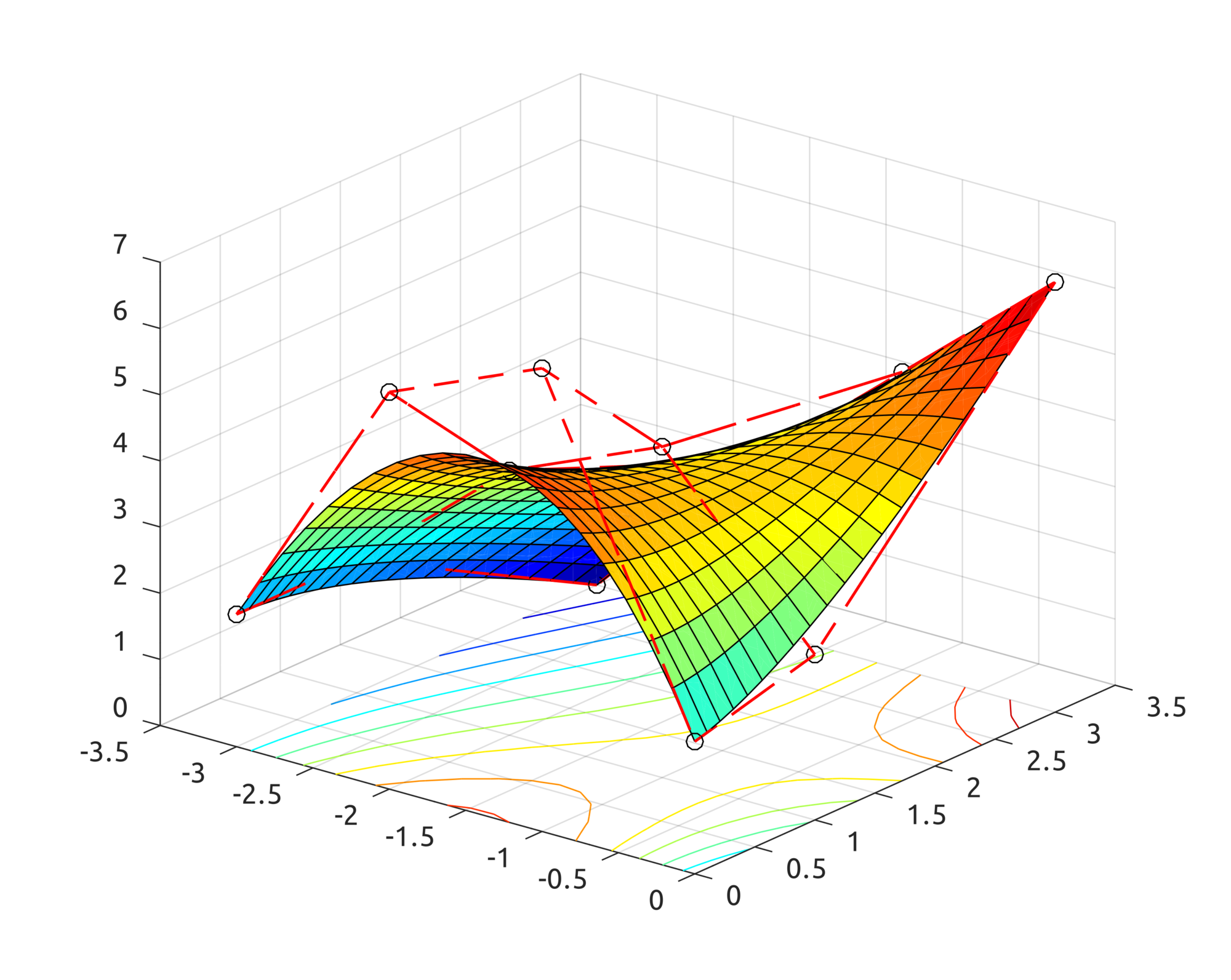
By using the defined basis functions, data defined in
https://github.com/carlonluca/isogeometric-analysis/blob/master/3.4/defineBsplineRing.m can draw a shape similar to a ring:
Note that this is not yet a toroid.
TypeScript Implementation
A TypeScript implementation is also present in the repo. With a simple code like this: