The main topic of the dissertation is not the Finite Element Method (FEM) actually, but the first and the second chapters present it and I wrote a basic implementation that works for 1D problems here: https://github.com/carlonluca/isogeometric-analysis/blob/master/2.3/drawFEM1DExample.m. The first example uses the implementation to compute an approximation using FEM.
Problem
In the code, the first example solves the differential equation:$$\left\{ \begin{array}{ll} \frac{d^{2}u(x)}{dx^{2}}=10 & \forall x\in\Omega=\left(0,1\right)\\ u(x)=0 & x=0\\ u(x)=1 & x=1 \end{array}\right.$$
Exact solution
It is possible to find an exact solution by integrating both parts twice:$$\iint_{\Omega}u''(x)dxdx=\iint_{\Omega}10dxdx\Rightarrow u(x)=5x^{2}+c_{1}x+c_{2}$$
The solution of the system:
$$\left\{ \begin{array}{ll} u(x)=5x^{2}+c_{1}x+c_{2} & \forall x\in\Omega=\left(0,1\right)\\ u(x)=0 & x=0\\ u(x)=1 & x=1 \end{array}\right.$$
is the exact solution to the problem:
$$u(x)=x\cdot(5x-4)$$
Weak Formulation
To calculate the weak formulation we need to first define a Dirichlet lift, as the boundary conditions are non-homogeneous:$$u(x)=\gamma(x)+v(x)\Rightarrow(\gamma(x)+v(x))''=10$$
Multiply by a test function $\varphi\in C_{0}^{\infty}(\Omega)$:
$$(\gamma(x)+v(x))''\cdot\varphi(x)=10\cdot\varphi(x)$$
Now integrate both parts:
$$\int_{\Omega}(\gamma(x)+v(x))''\cdot\varphi(x)dx=\int_{\Omega}10\cdot\varphi(x)dx$$
Using the technique of integration by parts:
$$\int_{a}^{b}u(x)v'(x)dx=\left[u(x)v(x)\right]_{a}^{b}-\int_{a}^{b}u'(x)v(x)dx$$
we can get to:
$$\left[\varphi(x)\left(\gamma(x)+v(x)\right)'\right]_{\Omega}-\int_{\Omega}\varphi'(x)\left(\gamma(x)+v(x)\right)'dx=\int_{\Omega}10\varphi(x)dx$$
$\varphi$ is a distribution and it therefore vanishes on the boundary:
$$-\int_{\Omega}\varphi'(x)\left(\gamma(x)+v(x)\right)'dx=\int_{\Omega}10\varphi(x)dx$$
It is now possible to define the two terms:
$$a(v,\varphi)=\int_{\Omega}\varphi'(x)v'(x)dx$$ $$l(\varphi)=-\int_{\Omega}\left(\varphi'(x)\gamma'(x)+10\varphi(x)\right)dx$$
Galerkin Method
At this point, the Galerkin method can be applied if we accept to look for an approximate solution in a space $V_{n}$ of dimension $dim(V_{n})=n$. Thus, assuming $\left\{ v_{i}\right\} _{i=0}^{n-1}$ is a basis for $V_{n}$, then we can write our approx solution:$$\tilde{v}(x)=\sum_{i=0}^{n-1}\bar{v}_{i}\cdot v_{i}(x)$$
where $\left\{ \bar{v}_{i}\right\} _{i=0}^{n-1}$ are coefficients of the linear combination.
We can create a linear system with $n$ independent equations that can be written in matrix form as:
$$\boldsymbol{S}_{n}\cdot\boldsymbol{\Upsilon}_{n}=\boldsymbol{F}_{n}$$
where:
$$\boldsymbol{S}_{n}=\left[\int_{0}^{1}v_{i}v_{j}dx\right]_{i,j=0}^{n-1}$$ $$\boldsymbol{\Upsilon}_{n}=\left[\bar{v}_{i}\right]_{i=0}^{n-1}$$ $$\boldsymbol{F}_{n}=\left[-\int_{0}^{1}\left(v_{i}'(x)\gamma'(x)+10\gamma(x)\right)dx\right]_{i=0}^{n-1}$$
The basis functions $\left\{ v_{i}\right\} _{i=0}^{n-1}$ can be chosen according to the needs. In the example, simple roof functions are used: https://github.com/carlonluca/isogeometric-analysis/blob/master/2.3/computePhi.m and https://github.com/carlonluca/isogeometric-analysis/blob/master/2.3/computeDphi.m (note that nomenclature in the code is slightly different). Different approximations can be achieved with a different basis for the space $V_{n}$.
A possible choice for the Dirichlet lift is:
$$\gamma(x)=0\cdot v_{0}(x)+1\cdot v_{n-1}(x)$$
which is the one that is used in the example implementation.
Result
The example script solves the problem for $n=2,...,7$. As expected with FEM, the approximation is exact at the nodes. By increasing the dimension of the space where the solution is to be found, the approximation gets closer to the exact curve.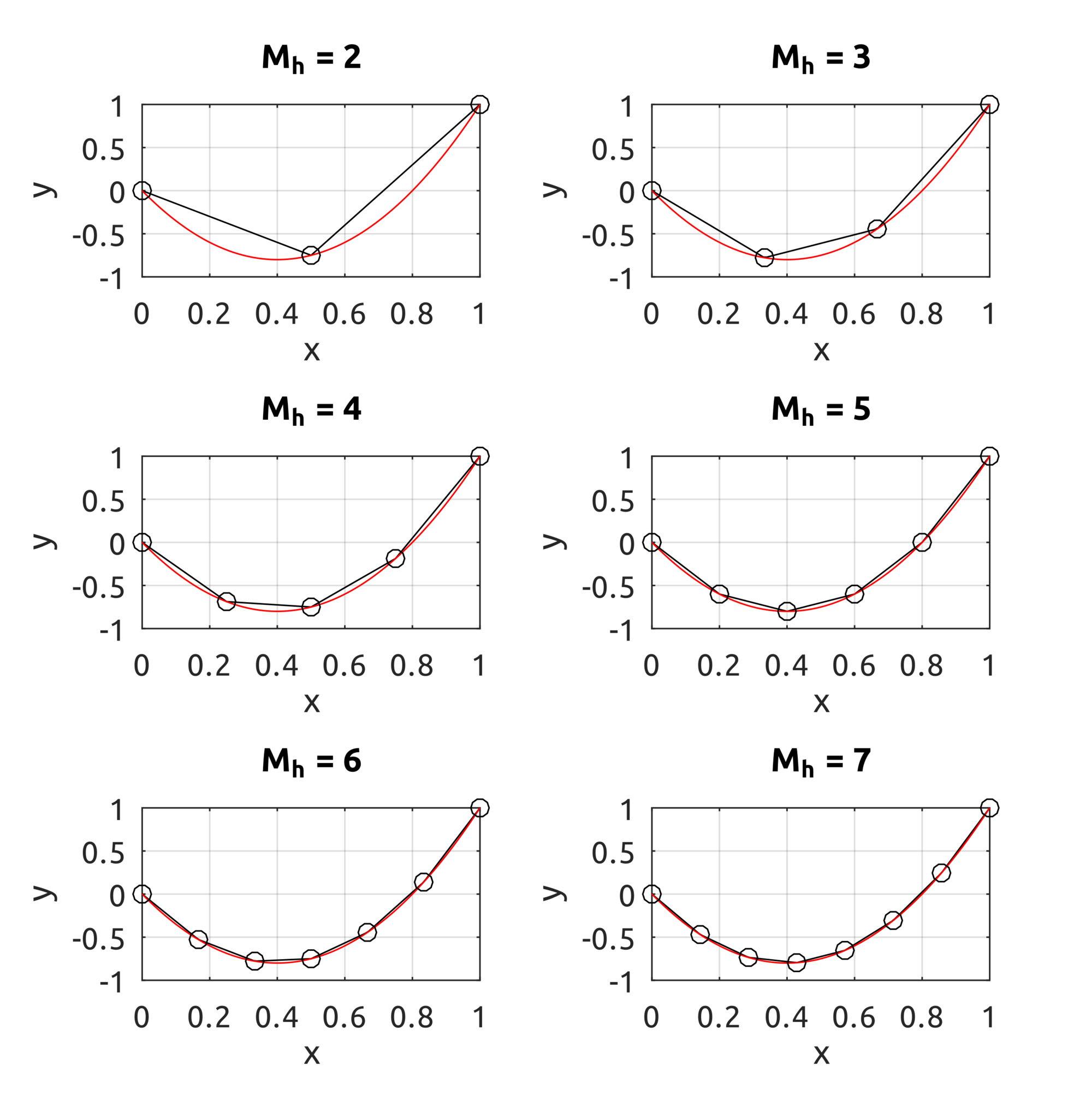
Lagrange Polynomials
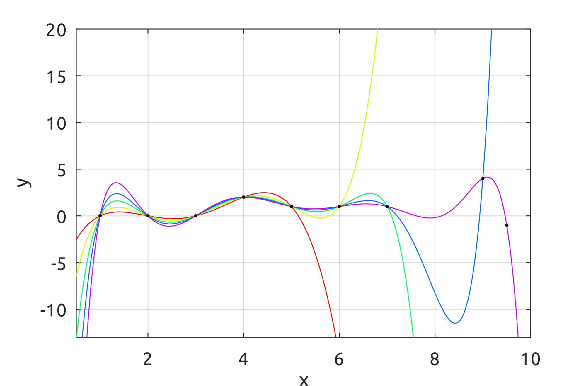
In the previous implementation, roof functions were used. It is possible to use piecewise-polynomials of higher order. One possible implementation is Lagrange polynomials.$$l_{Lag,i}\left(\xi\right)={\displaystyle \prod_{1\leq j\leq p_{m}+1,j\neq i}\dfrac{\left(\xi-y_{j}\right)}{\left(y_{i}-y_{j}\right)},\;i=1,2,\ldots,p_{m}+1}$$
In the repo there is a sample implementation. The demo draws Lagrange polynomials interpolating an increasing number of points: