Isogeometric Analysis: Bezier Curves and Surfaces in Octave and TypeScript

While working on my sample IGA implementation here https://github.com/carlonluca/isogeometric-analysis, I found myself in need of defining and implementing the math structures used to define the domain and the solution space. This means that I had to implement various algorithms to define structures like Bezier, B-spline, NURBS and T-spline. So this is a quick intro to Bezier curves and surfaces with a couple of implementations.

Power Basis

A simple math structure to handle curves and surfaces is the power basis representation. Power basis representation uses polynomials, which are fast to compute and simple to handle.
A $n^{th}$-degree power basis curve can be defined in the parametric space as:

$$\begin{eqnarray*} \boldsymbol{C}\left(\xi\right) & = & \left(x\left(\xi\right),y\left(\xi\right),z\left(\xi\right)\right)\\ & = & \sum_{i=0}^{n}\boldsymbol{a}_{i}\xi^{i}\\ & = & \left(\left[\boldsymbol{a}_{i}\right]_{i=0}^{n}\right)^{T}\left[\xi^{i}\right]_{i=0}^{n}, \end{eqnarray*}$$

where the functions $\xi^{i}$ are the basis (or blending) functions. Using the tensor product scheme we can also define a power basis surface:

$$\begin{eqnarray*} \boldsymbol{S}\left(\xi,\eta\right) & = & \left(x\left(\xi,\eta\right),y\left(\xi,\eta\right),z\left(\xi,\eta\right)\right)\\ & = & \sum_{i=0}^{n}\sum_{j=0}^{m}\boldsymbol{a}_{i,j}\xi^{i}\eta^{j}\\ & = & \left(\left[\xi^{i}\right]_{i=0}^{n}\right)^{T}\left[\boldsymbol{a}_{i,j}\right]_{i,j=0}^{i=n,j=m}\left[\eta^{j}\right]_{j=0}^{m} \end{eqnarray*}$$

where:

$$ \left\{ \begin{array}{l} \boldsymbol{a}_{i,j}=\left(x_{i,j},y_{i,j},z_{i,j}\right)\\ b\leq\xi\leq c\\ d\leq\eta\leq e \end{array}\right.$$

Bezier

Bezier curves do not increase the space of curves representable by the power basis form, but introduce the concept of control point. Control points convey a clear geometrical meaning, which is very useful during the design process. So, a $n^{th}$-degree Bezier curve is defined as:

$$\boldsymbol{C}\left(\xi\right)=\sum_{i=0}^{n}B_{i}^{n}\left(\xi\right)\boldsymbol{P}_{i},\;a\leq\xi\leq b$$

where $\boldsymbol{P}_{i}$ represents the $i^{th}$ control point and:

$$B_{i}^{n}\left(\xi\right)=\frac{n!\cdot\xi^{i}\left(1-\xi\right)^{n-i}}{i!\cdot\left(n-i\right)!}$$

is the $i^{th}$ basis function (also known as Bernstein polynomial). With the tensor product scheme, we can also define a Bezier surface with:

$$\boldsymbol{S}\left(\xi,\eta\right)=\sum_{i=0}^{n}\sum_{j=0}^{m}B_{i}^{n}\left(\xi\right)B_{j}^{m}\left(\eta\right)\boldsymbol{P}_{i,j},\;\left\{ \begin{array}{l} a\leq\xi\leq b\\ c\leq\eta\leq d \end{array}\right.$$

Octave Implementation

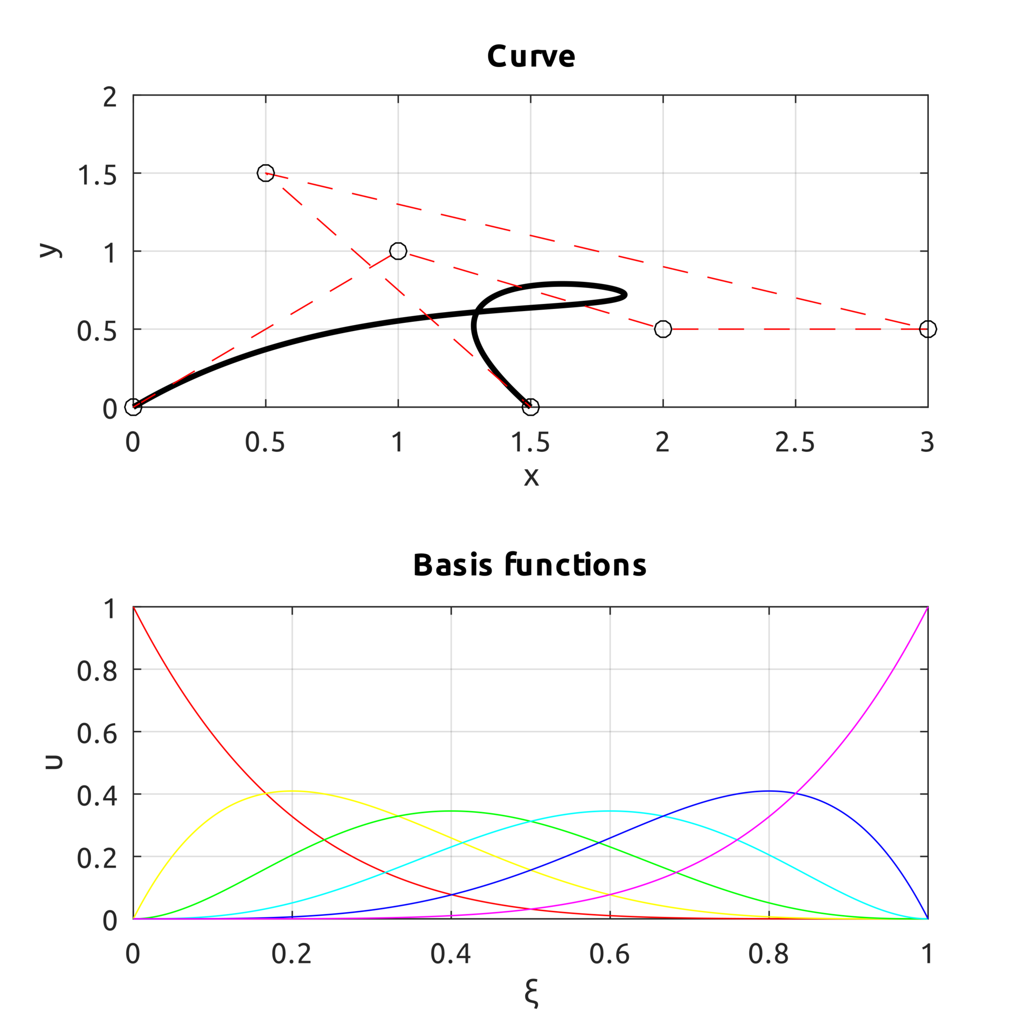
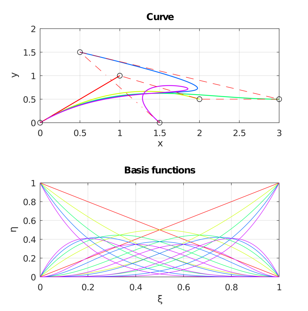
In the repo https://github.com/carlonluca/isogeometric-analysis, you can find a basic implementation of Bezier curves and surfaces written for Octave (and Matlab) in: https://github.com/carlonluca/isogeometric-analysis/tree/master/3.3. The implementation is tested with a few examples. For example, given these control points:

$$\boldsymbol{P}_{0}=\left(0,0\right),\;\boldsymbol{P}_{1}=\left(1,1\right),\;\boldsymbol{P}_{2}=\left(2,0.5\right)$$ $$\boldsymbol{P}_{3}=\left(3,0.5\right),\;\boldsymbol{P}_{4}=\left(0.5,1.5\right),\;\boldsymbol{P}_{5}=\left(1.5,0\right)$$

we can get to this result by using the computeBezier.m script:

We can also define the curve in the 3D space. For example these control points:

$$\boldsymbol{P}_{0}=\left(0,0,0\right),\;\boldsymbol{P}_{1}=\left(1,1,1\right),\;\boldsymbol{P}_{2}=\left(2,0.5,0\right)$$ $$\boldsymbol{P}_{3}=\left(3,0.5,0\right),\;\boldsymbol{P}_{4}=\left(0.5,1.5,0\right),\;\boldsymbol{P}_{5}=\left(1.5,0,1\right)$$

lead to this result:

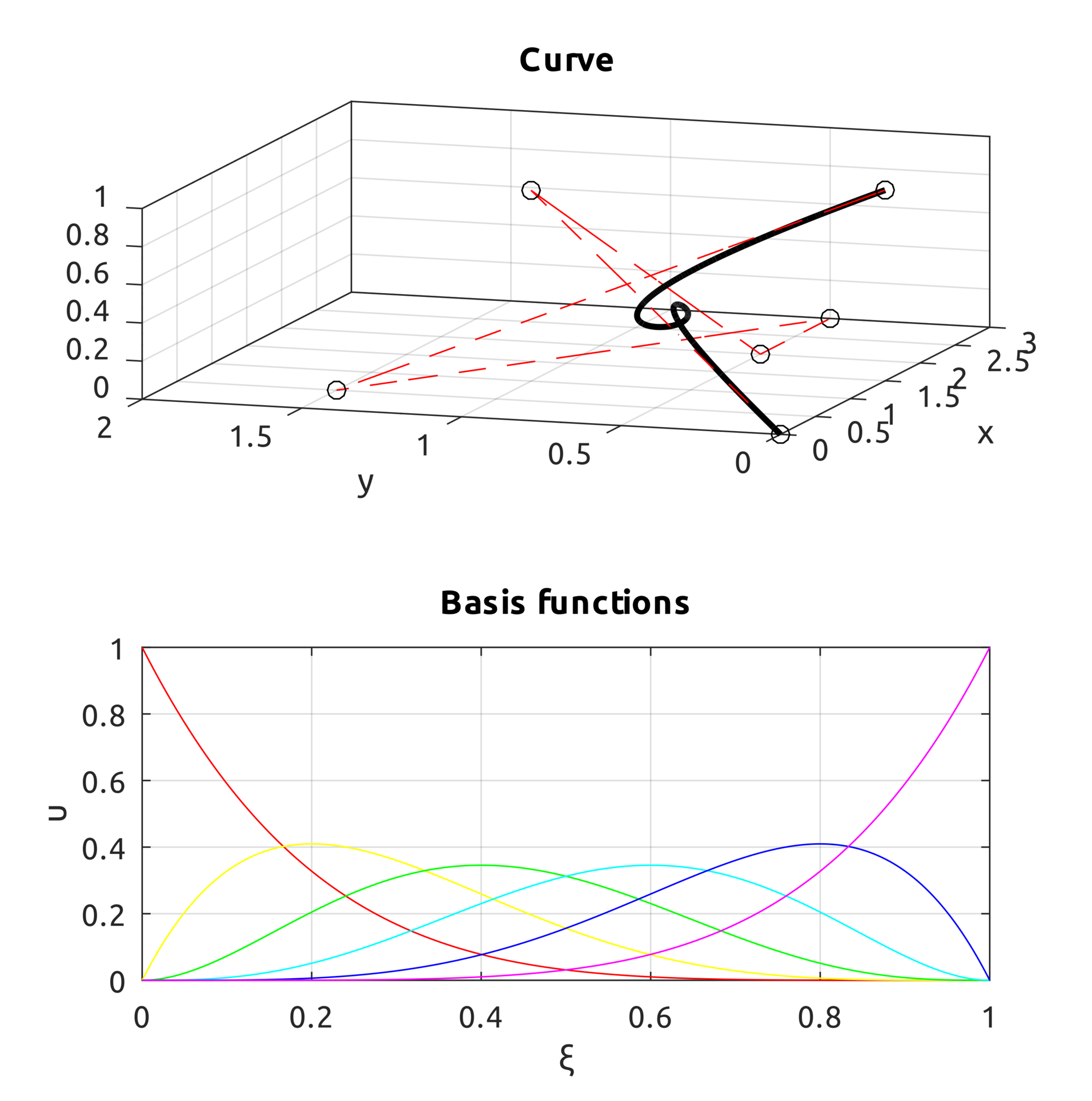
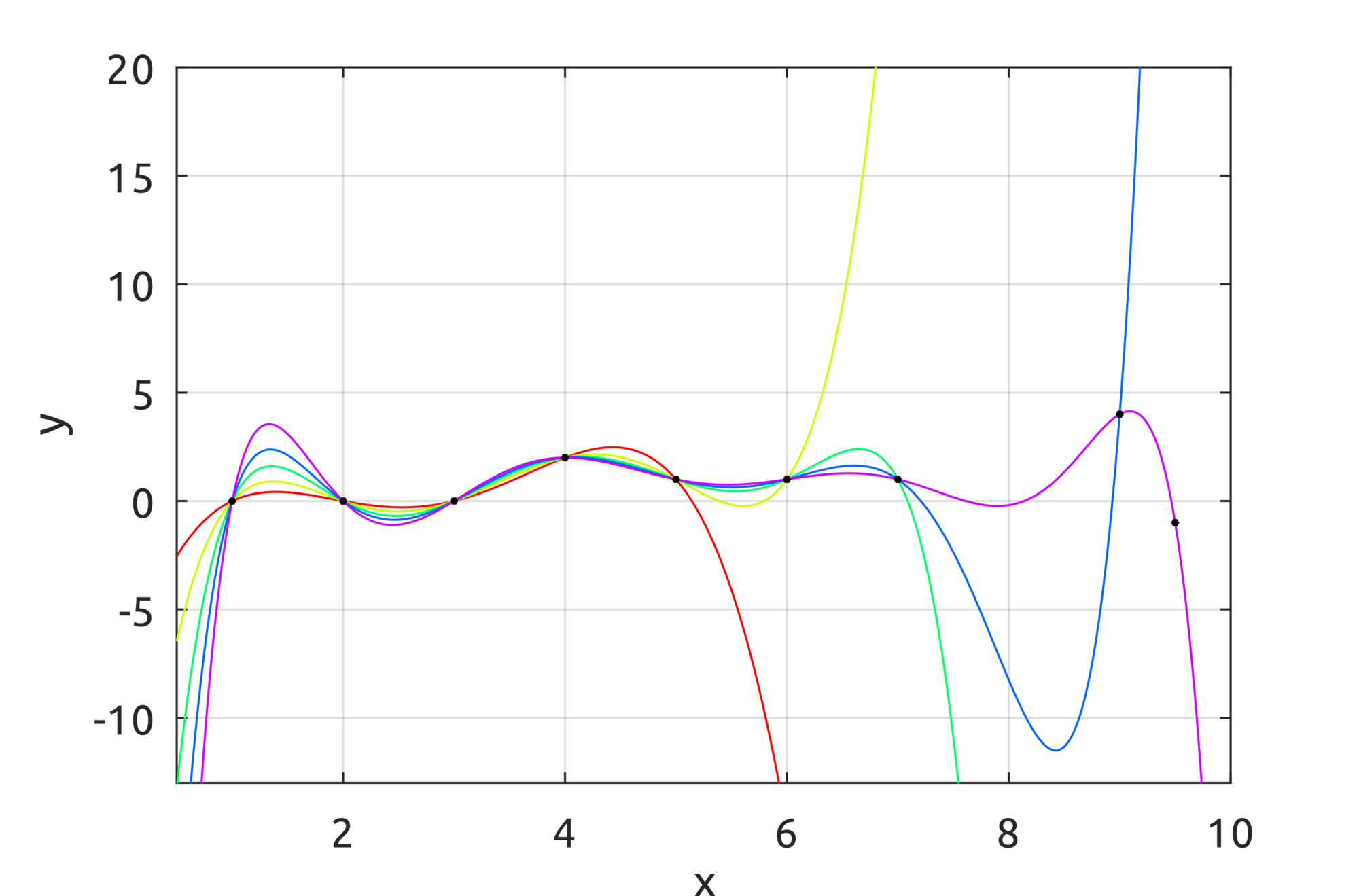
It may also be interesting to see what happens to a curve when a new control point is added to the previous one:

Another example is provided for Bezier surfaces. From these control points:

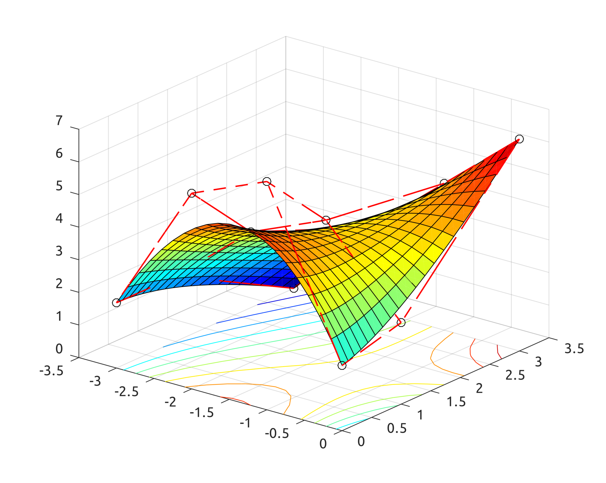
$$\boldsymbol{P}_{0}=\left(-3,0,2\right),\;\boldsymbol{P}_{1}=\left(-2,0,6\right),\;\boldsymbol{P}_{2}=\left(-1,0,7\right),\boldsymbol{P}_{3}=\left(0,0,2\right)$$ $$\boldsymbol{P}_{4}=\left(-3,1,2\right),\;\boldsymbol{P}_{5}=\left(-2,1,4\right),\;\boldsymbol{P}_{6}=\left(-1,1,5\right),\;\boldsymbol{P}_{7}=\left(0,1,2.5\right)$$ $$\boldsymbol{P}_{8}=\left(-3,3,0\right),\;\boldsymbol{P}_{9}=\left(-2,3,2.5\right),\;\boldsymbol{P}_{10}=\left(-1,3,4.5\right),\;\boldsymbol{P}_{11}=\left(0,3,6.5\right)$$

this is what the algorithms produce:

Typescript Implementation

What about a browser implemenation? The above algorithms can clearly be implemented in a browser, so this is an attempt written in TypeScript: https://github.com/carlonluca/isogeometric-analysis/tree/master/ts/src/bezier. The BezierCurve object can be used to draw a plot of the first examples:

Isogeometric Analysis and Finite Element Method

It's been some years since I completed my dissertation on FEM and Isogeometric Analysis, but I realised I never had the time to organise my code properly and archive it. So I archived a part of it in a new repo here: https://github.com/carlonluca/isogeometric-analysis. It may be useful for someone studying the topic.

The main topic of the dissertation is not the Finite Element Method (FEM) actually, but the first and the second chapters present it and I wrote a basic implementation that works for 1D problems here: https://github.com/carlonluca/isogeometric-analysis/blob/master/2.3/drawFEM1DExample.m. The first example uses the implementation to compute an approximation using FEM.

Problem

In the code, the first example solves the differential equation:

$$\left\{ \begin{array}{ll} \frac{d^{2}u(x)}{dx^{2}}=10 & \forall x\in\Omega=\left(0,1\right)\\ u(x)=0 & x=0\\ u(x)=1 & x=1 \end{array}\right.$$

Exact solution

It is possible to find an exact solution by integrating both parts twice:

$$\iint_{\Omega}u''(x)dxdx=\iint_{\Omega}10dxdx\Rightarrow u(x)=5x^{2}+c_{1}x+c_{2}$$

The solution of the system:

$$\left\{ \begin{array}{ll} u(x)=5x^{2}+c_{1}x+c_{2} & \forall x\in\Omega=\left(0,1\right)\\ u(x)=0 & x=0\\ u(x)=1 & x=1 \end{array}\right.$$

is the exact solution to the problem:

$$u(x)=x\cdot(5x-4)$$

Weak Formulation

To calculate the weak formulation we need to first define a Dirichlet lift, as the boundary conditions are non-homogeneous:

$$u(x)=\gamma(x)+v(x)\Rightarrow(\gamma(x)+v(x))''=10$$

Multiply by a test function $\varphi\in C_{0}^{\infty}(\Omega)$:

$$(\gamma(x)+v(x))''\cdot\varphi(x)=10\cdot\varphi(x)$$

Now integrate both parts:

$$\int_{\Omega}(\gamma(x)+v(x))''\cdot\varphi(x)dx=\int_{\Omega}10\cdot\varphi(x)dx$$

Using the technique of integration by parts:

$$\int_{a}^{b}u(x)v'(x)dx=\left[u(x)v(x)\right]_{a}^{b}-\int_{a}^{b}u'(x)v(x)dx$$

we can get to:

$$\left[\varphi(x)\left(\gamma(x)+v(x)\right)'\right]_{\Omega}-\int_{\Omega}\varphi'(x)\left(\gamma(x)+v(x)\right)'dx=\int_{\Omega}10\varphi(x)dx$$

$\varphi$ is a distribution and it therefore vanishes on the boundary:

$$-\int_{\Omega}\varphi'(x)\left(\gamma(x)+v(x)\right)'dx=\int_{\Omega}10\varphi(x)dx$$

It is now possible to define the two terms:

$$a(v,\varphi)=\int_{\Omega}\varphi'(x)v'(x)dx$$ $$l(\varphi)=-\int_{\Omega}\left(\varphi'(x)\gamma'(x)+10\varphi(x)\right)dx$$

Galerkin Method

At this point, the Galerkin method can be applied if we accept to look for an approximate solution in a space $V_{n}$ of dimension $dim(V_{n})=n$. Thus, assuming $\left\{ v_{i}\right\} _{i=0}^{n-1}$ is a basis for $V_{n}$, then we can write our approx solution:

$$\tilde{v}(x)=\sum_{i=0}^{n-1}\bar{v}_{i}\cdot v_{i}(x)$$

where $\left\{ \bar{v}_{i}\right\} _{i=0}^{n-1}$ are coefficients of the linear combination.
We can create a linear system with $n$ independent equations that can be written in matrix form as:

$$\boldsymbol{S}_{n}\cdot\boldsymbol{\Upsilon}_{n}=\boldsymbol{F}_{n}$$

where:

$$\boldsymbol{S}_{n}=\left[\int_{0}^{1}v_{i}v_{j}dx\right]_{i,j=0}^{n-1}$$ $$\boldsymbol{\Upsilon}_{n}=\left[\bar{v}_{i}\right]_{i=0}^{n-1}$$ $$\boldsymbol{F}_{n}=\left[-\int_{0}^{1}\left(v_{i}'(x)\gamma'(x)+10\gamma(x)\right)dx\right]_{i=0}^{n-1}$$

The basis functions $\left\{ v_{i}\right\} _{i=0}^{n-1}$ can be chosen according to the needs. In the example, simple roof functions are used: https://github.com/carlonluca/isogeometric-analysis/blob/master/2.3/computePhi.m and https://github.com/carlonluca/isogeometric-analysis/blob/master/2.3/computeDphi.m (note that nomenclature in the code is slightly different). Different approximations can be achieved with a different basis for the space $V_{n}$.
A possible choice for the Dirichlet lift is:

$$\gamma(x)=0\cdot v_{0}(x)+1\cdot v_{n-1}(x)$$

which is the one that is used in the example implementation.

Result

The example script solves the problem for $n=2,...,7$. As expected with FEM, the approximation is exact at the nodes. By increasing the dimension of the space where the solution is to be found, the approximation gets closer to the exact curve.

Lagrange Polynomials

In the previous implementation, roof functions were used. It is possible to use piecewise-polynomials of higher order. One possible implementation is Lagrange polynomials.

$$l_{Lag,i}\left(\xi\right)={\displaystyle \prod_{1\leq j\leq p_{m}+1,j\neq i}\dfrac{\left(\xi-y_{j}\right)}{\left(y_{i}-y_{j}\right)},\;i=1,2,\ldots,p_{m}+1}$$

In the repo there is a sample implementation. The demo draws Lagrange polynomials interpolating an increasing number of points: