Saturday, August 21, 2021

Cross-building the Ubuntu Kernel for the Raspberry Pi 4 (arm64)

I recently had to rebuild the Ubuntu kernel for the Raspberry Pi pretty often to apply some patches. Building on the Pi is simple, but takes A LOT of hours and completely saturates the rpi4. Also, it means installing many dev packages, which I do not typically need. I also tried to do it on a development rpi3: took many hours, failed a few times because of insufficient RAM etc… It is a pain.

I therefore decided to try to cross-build it from my machine, which is not a Ubuntu machine at the moment. Quickest and simplest way I found is to use Docker. The result seems to work, so I decided to also provide the tools I created for myself here: https://github.com/carlonluca/docker-rpi-ubuntu-kernel.

Usage

The image only contains the tools and the libs needed to compile. The kernel itself and the script is provided externally. A workspace directory will contain both the kernel code to build and the output debian packages. With the following command the script is executed in the container and you should get your debs:
docker run --rm -it --name builder -v $PWD/workspace:/workspace \
    -v $PWD/build.sh:/workspace/build.sh carlonluca/docker-rpi-ubuntu-kernel:focal \
    /workspace/build.sh
The workspace directory must contain a src directory with the kernel, so you’ll have to create it yourself and then patch your kernel:
mkdir workspace
cd workspace
git clone https://git.launchpad.net/~ubuntu-kernel/ubuntu/+source/linux-raspi/+git/hirsute src
[apply needed patches]
The resulting packages can then be moved to the pi and installed with:
sudo dpkg -i *.deb
Hope this tool can be useful! Bye ;-)

Tuesday, August 17, 2021

Docker Image for Qt Development and Continuous Integration on x64 and arm64

Intro

It happens from time to time that I would benefit from having a simple Docker image with all the deps needed to build and run Qt apps on specific Qt versions. For instance, I may need to build some binary on Mac OS for Linux or I may need to have an image for some continuous integration system.

Problem

I had a look around and there are quite a few projects: some do not provide an arm build, some rely on the Qt official installer, that is a bit tricky to automate and tends to change often, some rely on distro-provided packages, that do not provide every version etc… I’d prefer to have a solid build procedure to build images for any Qt version I want. Also, my CI system runs on arm64, so I’d need a multiarch image, and therefore two different Qt builds. I thought it could be simpler to just build Qt on-the-fly in a Dockerfile but… turned out it is not exactly simple.

Solution

At first I created a Dockerfile to:
  1. install all the needed deps on Ubuntu focal;
  2. download Qt sources;
  3. configure;
  4. build;
  5. install;
  6. cleanup.
This proved to be a simple solution, but building Qt for arm on qemu or building on arm took way too much. So I though of a different solution. I created two images:
With the first image Qt can be built and cross-built in a few hours for both x64 and arm64, directly on x64. The builds are then injected into a second multiarch image. This is way faster than building on qemu.

Only one problem left: in Qt 5, crossbuilding Qt results in some Qt tools like qmake to be built for the host arch, which is unacceptable in this case. So, in the second image, a build of the only qtbase module is also needed to build arm64 binaries. Qt 6 works differently instead.

Result

The code to build Qt and all the images are available at: https://github.com/carlonluca/docker-qt.
The image to use for app development is available at: https://hub.docker.com/repository/docker/carlonluca/qt-dev.

Continuous Integration on GitLab with Qt

An example of usage of the dev image is running continuous integration and unit tests on your code on Jenkins or GitLab. For example, I can now run my unit tests in my GitLab instance running on Raspberry Pi 4 with the following code (taken from my project https://github.com/carlonluca/lqobjectserializer):
variables:

GIT_SUBMODULE_STRATEGY: recursive

stages:
  - test_qt5
  - test_qt6

Test_qt5:
  stage: test_qt5
  image:
    name: "carlonluca/qt-dev:5.15.2"
    entrypoint: [""]
  script:
    - cd LQObjectSerializerTest
    - mkdir build
    - cd build
    - cmake ../qt5
    - make
    - ./LQObjectSerializerTest
    - ./LGithubTestCase

Test_qt6:
  stage: test_qt6
  image:
    name: "carlonluca/qt-dev:6.1.2"
    entrypoint: [""]
  script:
    - cd LQObjectSerializerTest
    - mkdir build
    - cd build
    - cmake ../qt6
    - make
    - ./LQObjectSerializerTest
    - ./LGithubTestCase


These images are still experimental though.
Have fun 😉

Bye!

Sunday, July 25, 2021

Dark Theme for MediaWiki in Docker

I recently started to use MediaWiki as a way to store personal information, notes, links etc... It is comfortable to have all that info with me, properly structured, immediately editable online regardless of the operating system and versioned. Adding an instance of MediaWiki to an existent setup is straightforward, and I like to do it with docker. The official docker image of MediaWiki is already multiarch, so I could add it to my Raspberry Pi quickly. Default MediaWiki includes a light theme, but does not seem to include a dark theme. This is where this project by Martynov Maxim comes to help: https://github.com/dolfinus/DarkVector. You'll have to add it to your MediaWiki container and select it for your users.

Keeping MediaWiki up to date (and only usable through HTTPS) is important for security reasons (https://www.mediawiki.org/wiki/Manual:Security) so I created my own MediaWiki multiarch image including that theme by default. You can freely use it: https://hub.docker.com/repository/docker/carlonluca/darkmediawiki. I use it successfully on my aarch64 installation. This is the result:
Refreshing the image is almost effertless thanks to the CI/CD capabilities of GitLab.
For more info refer to the GitHub project: https://github.com/carlonluca/darkmediawiki-docker. Have fun ;-)

Sunday, July 11, 2021

Isogeometric Analysis: NURBS curves and surfaces in Octave and TypeScript

In this blog post I wrote some notes about B-splines. There are however important classes of curves and surfaces that cannot be represented by piecewise-polynomials like circles, ellipses etc... NURBS come to the rescue.

NURBS curves

NURBS is a generalization of B-splines where basis functions are defined with piecewise-rational polynomials. Again the parametric domain is split into multiple ranges by using a knot vector. The general definition is:

$$\boldsymbol{C}\left(\xi\right)=\sum_{i=0}^{n}R_{i}^{p}\left(\xi\right)\boldsymbol{P}_{i},\;a\leq\xi\leq b$$
$\boldsymbol{P}_{i}$ are the control points and the functions $R_{i}^{p}$ are the NURBS basis functions, defined as:

$$R_{i}^{p}\left(\xi\right)=\dfrac{N_{i}^{p}\left(\xi\right)w_{i}}{{\displaystyle\sum_{i=0}^{n}N_{i}^{p}\left(\xi\right)w_{i}}},\;a\leq\xi\leq b,$$
where the functions $N_i^{p}$ are the B-spline basis functions (defined here):

$$N_{i}^{0}\left(\xi\right)=\left\{ \begin{array}{ll}1, & \xi_{i}\leq\xi<\xi_{i+1}\\0,&\text{otherwise}\end{array}\right.,a\leq\xi\leq b$$ $$N_{i}^{p}\left(\xi\right)=\frac{\xi-\xi_{i}}{\xi_{i+p}-\xi_{i}}\cdot N_{i}^{p-1}\left(\xi\right)+\frac{\xi_{i+p+1}-\xi}{\xi_{i+p+1}-\xi_{i+1}}\cdot N_{i+1}^{p-1}\left(\xi\right),a\leq\xi\leq b$$
and the values $w_i$'s are known as weights. The knot vector has the same definition given for B-spline curves:

$$\Xi=\left[\underset{p+1}{\underbrace{a,\ldots,a}},\xi_{p+1},\ldots\xi_{n},\underset{p+1}{\underbrace{b,\ldots,b}}\right],\;\left|\Xi\right|=n+p+2,$$

NURBS surfaces

By using the tensor product we can obtain definitions for NURBS in spaces of higher dimension. For surfaces, given the knot vectors:

$$\Xi=\left[\underset{p+1}{\underbrace{a_{0},\ldots,a_{0}}},\xi_{p+1},\ldots,\xi_{n},\underset{p+1}{\underbrace{b_{0},\ldots,b_{0}}}\right],\left|\Xi\right|=n+p+2$$ $$H=\left[\underset{q+1}{\underbrace{a_{1},\ldots,a_{1}}},\xi_{q+1},\ldots,\xi_{m},\underset{q+1}{\underbrace{b_{1},\ldots,b_{1}}}\right],\left|H\right|=m+q+2$$
a NURBS surface can be defined as:

$$\boldsymbol{S}\left(\xi,\eta\right)=\sum_{i=0}^{n}\sum_{j=0}^{m}R_{i,j}^{p,q}\left(\xi,\eta\right)\boldsymbol{P}_{i,j},\;\left\{ \begin{array}{c}a_{0}\leq\xi\leq b_{0}\\a_{1}\leq\eta\leq b_{1}\end{array}\right.$$
where:

$$R_{i,j}^{p,q}\left(\xi,\eta\right)=\dfrac{N_{i}^{p}\left(\xi\right)N_{j}^{q}\left(\eta\right)w_{i,j}}{{\displaystyle \sum_{\hat{i}=0}^{n}\sum_{\hat{j}=0}^{m}N_{\hat{i}}^{p}\left(\xi\right)N_{\hat{j}}^{q}\left(\eta\right)w_{\hat{i},\hat{j}}}},\;\left\{ \begin{array}{c}a_{0}\leq\xi\leq b_{0}\\a_{1}\leq\eta\leq b_{1}\end{array}\right.$$
and $w_{i,j}$ is the weight.

Homogeneous Coordinates

The implementations found in the repo do not directly implement the summations above, but use instead homogeneous coords to make calculations simpler. Let's consider the general form of a B-spline curve:

$$\boldsymbol{C}\left(\xi\right)=\sum_{i=0}^{n}N_{i}^{p}\left(\xi\right)\boldsymbol{P}_{i},\;a\leq\xi\leq b$$
Control points $\boldsymbol{P}_i$ can be written in homogeneous coords like this:

$$\boldsymbol{P}_{i}^{w}=\left[\begin{array}{c} x_{i}\\ y_{i}\\ z_{i}\\ 1 \end{array}\right]$$
We can multiply each control point by a value $w_i\neq 0$, and the result would still represent the same point in the euclidean space. As a result, we can write:

$$\boldsymbol{C}^{w}\left(\xi\right)=\sum_{i=0}^{n}N_{i}^{p}\left(\xi\right)\cdot\left[\begin{array}{c} x_{i}w_{i}\\ y_{i}w_{i}\\ z_{i}w_{i}\\ w_{i} \end{array}\right]=\left[\begin{array}{c} \sum_{i=0}^{n}N_{i}^{p}\left(\xi\right)x_{i}w_{i}\\ \sum_{i=0}^{n}N_{i}^{p}\left(\xi\right)y_{i}w_{i}\\ \sum_{i=0}^{n}N_{i}^{p}\left(\xi\right)z_{i}w_{i}\\ \sum_{i=0}^{n}N_{i}^{p}\left(\xi\right)w_{i} \end{array}\right]$$
$\boldsymbol{C}^w(\xi)$ is therefore the original B-spline curve in homogeneous coords. Now we can map back it to the euclidean space:

$$\boldsymbol{C}\left(\xi\right)=\left[\begin{array}{c} \frac{\sum_{i=0}^{n}N_{i}^{p}\left(\xi\right)x_{i}w_{i}}{\sum_{i=0}^{n}N_{i}^{p}\left(\xi\right)w_{i}}\\ \frac{\sum_{i=0}^{n}N_{i}^{p}\left(\xi\right)y_{i}w_{i}}{\sum_{i=0}^{n}N_{i}^{p}\left(\xi\right)w_{i}}\\ \frac{\sum_{i=0}^{n}N_{i}^{p}\left(\xi\right)z_{i}w_{i}}{\sum_{i=0}^{n}N_{i}^{p}\left(\xi\right)w_{i}}\\ 1 \end{array}\right]$$
which yields:

$$\boldsymbol{C}\left(\xi\right)=\frac{\sum_{i=0}^{n}N_{i}^{p}\left(\xi\right)w_{i}\boldsymbol{P}_{i}}{\sum_{i=0}^{n}N_{i}^{p}\left(\xi\right)w_{i}}$$
This means that, moving to homogeneous coords, we can use a simpler form. Given:

$$\boldsymbol{P}_{i}^{w}=\left[\begin{array}{c} x_{i}w_{i}\\ y_{i}w_{i}\\ z_{i}w_{i}\\ w_{i} \end{array}\right]$$ we can write a NURBS curve as:

$$\boldsymbol{C}^{w}\left(\xi\right)=\sum_{i=0}^{n}N_{i}^{p}\left(\xi\right)\boldsymbol{P}_{i}^{w}$$
and a NURBS surface as:

$$\boldsymbol{S}^{w}\left(\xi,\eta\right)=\sum_{i=0}^{n}\sum_{j=0}^{m}N_{i}^{p}\left(\xi\right)N_{j}^{q}\left(\eta\right)\boldsymbol{P}_{i}^{w}$$
All the implementations in the repo use these simpler forms.

Octave Implementation

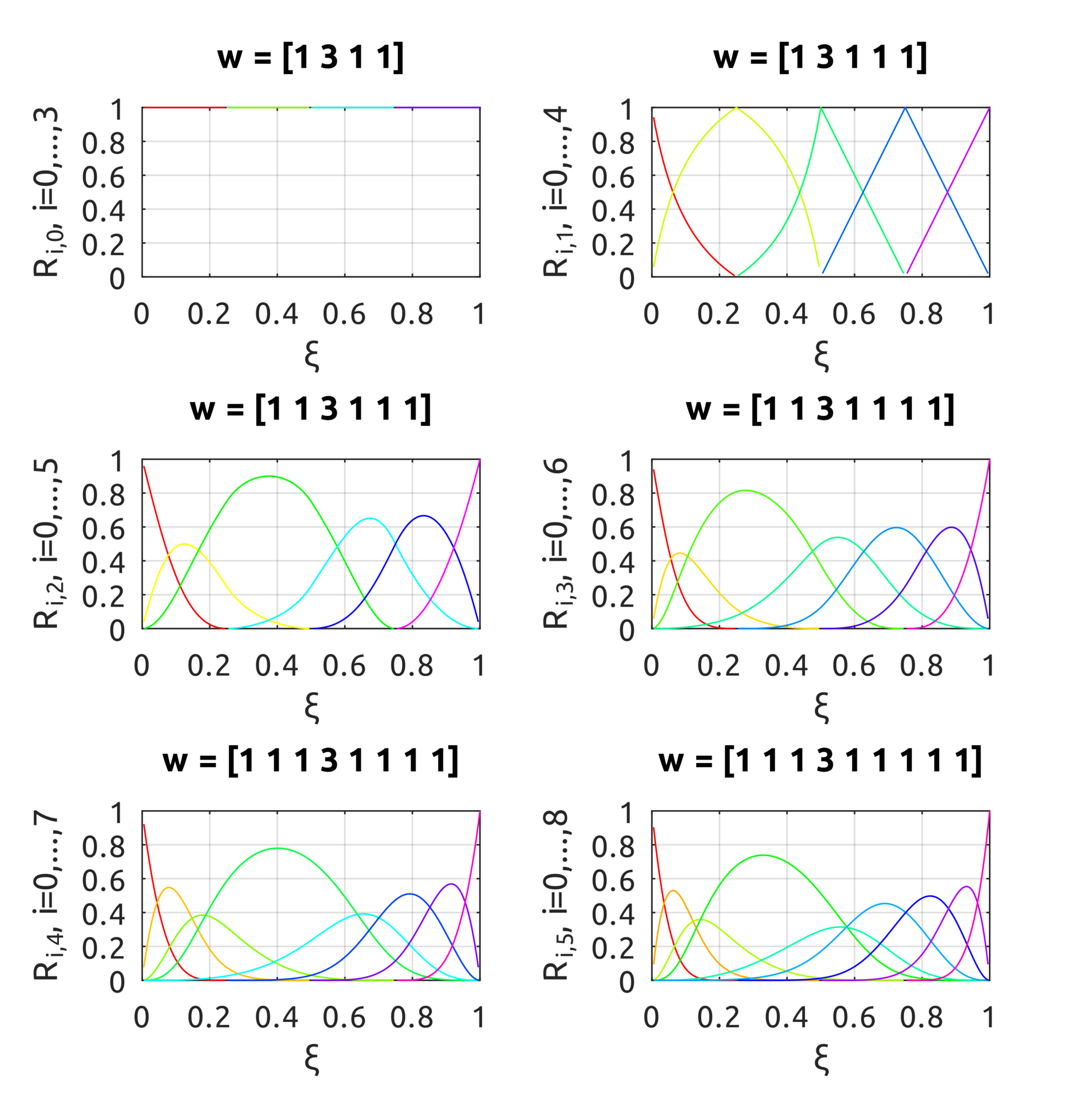
The computeNURBSBasisFun script can be used to compute NURBS basis functions. The drawNURBSBasisFunsP5 draws:

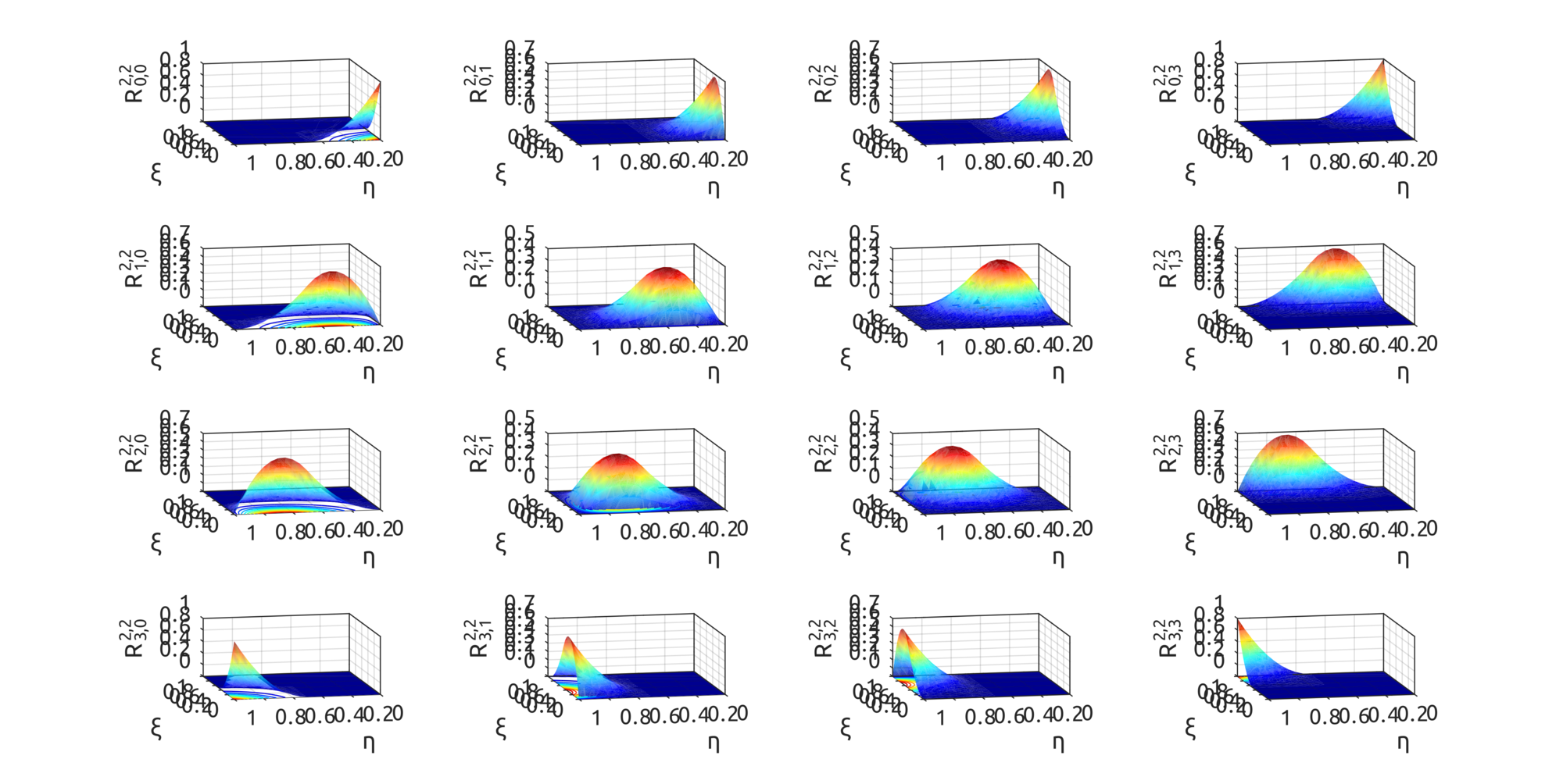
in the plots the effect of the weight is pretty clear. From top to bottom, the degree of the basis funs is increased over the knot vector $ Xi = [0.25, 0.5, 0.75]$.
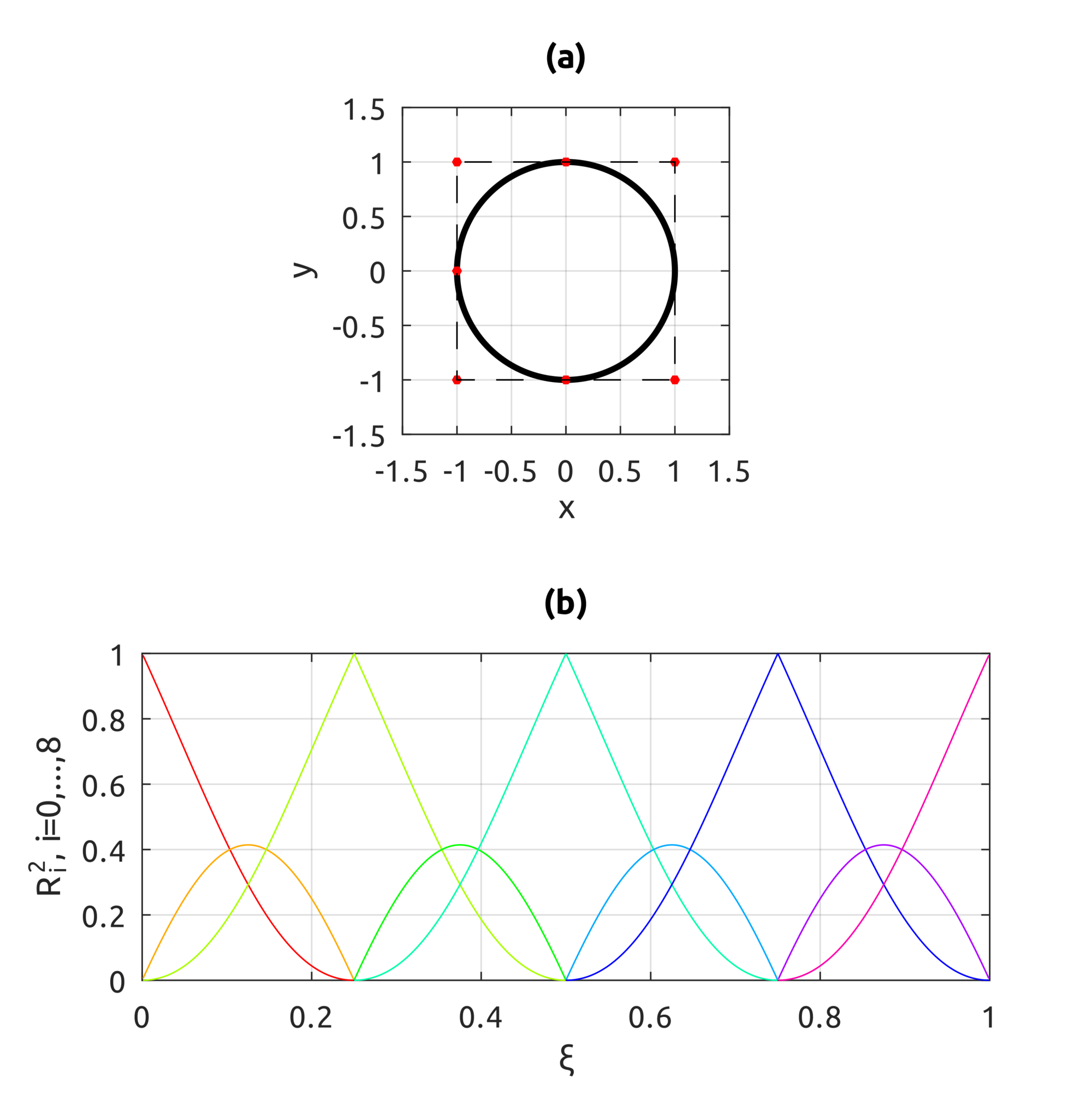
The computeNURBSCurvePoint script uses homogeneous coords to compute a NURBS curve using B-spline basis functions. We can build curves similar to what we could draw with B-splines but we can also draw circles:

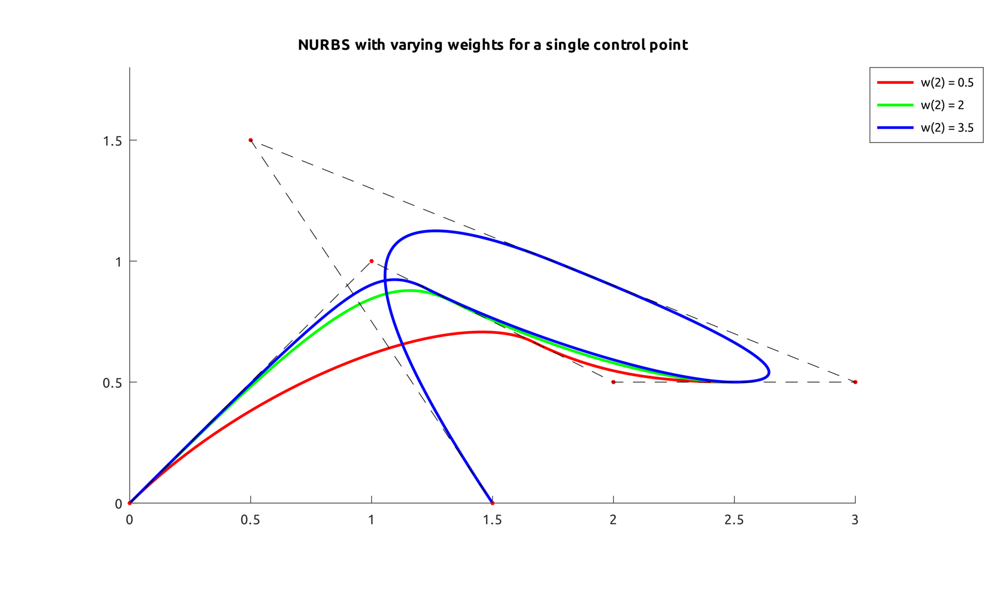
This is an example that shows what happens when a weight is increased on one point:

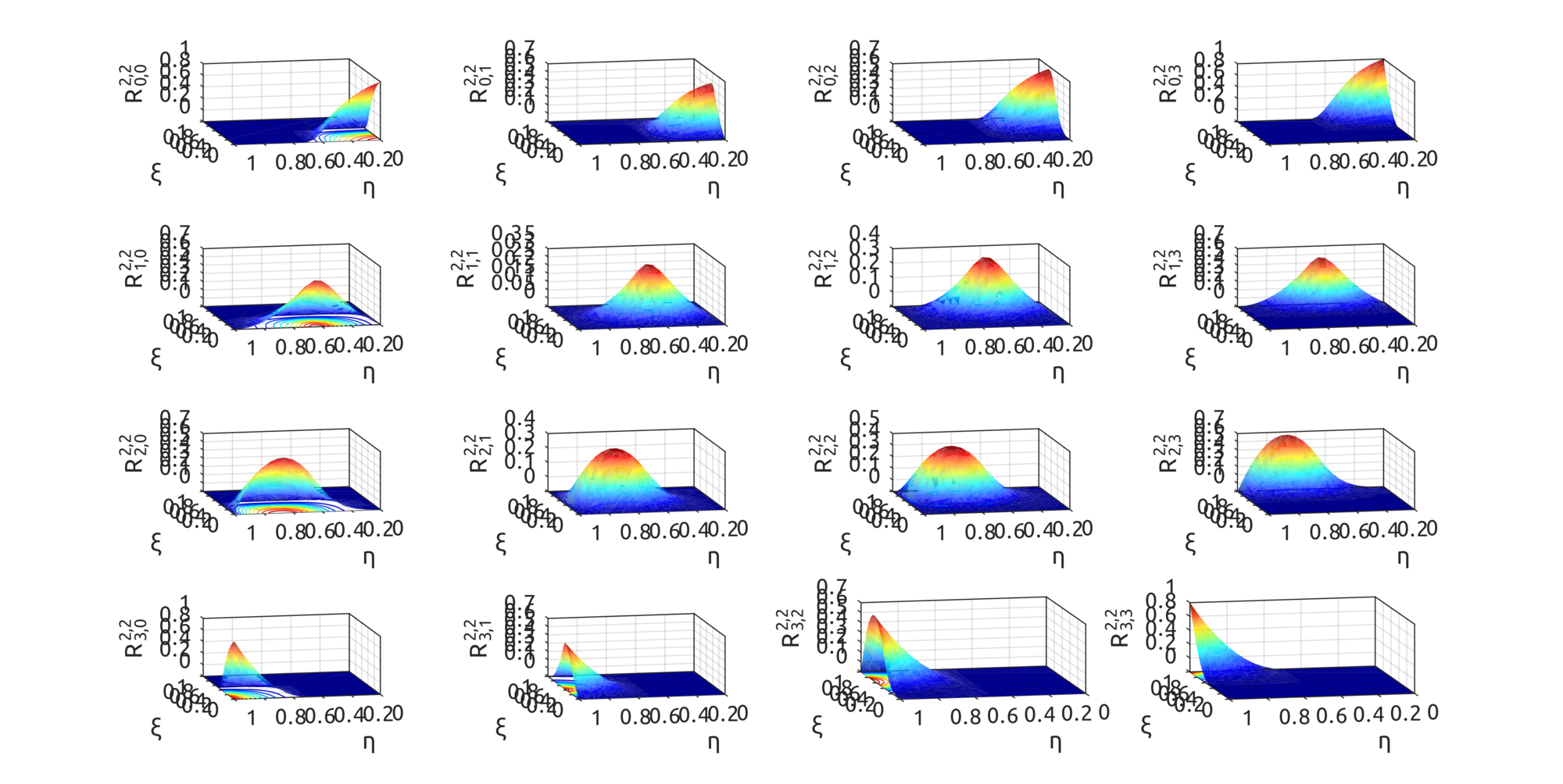
For NURBS surfaces instead we can draw bivariate basis functions. In these two examples, the first shows what happens when weights are all equal to 1, the second when weights are not all equal:


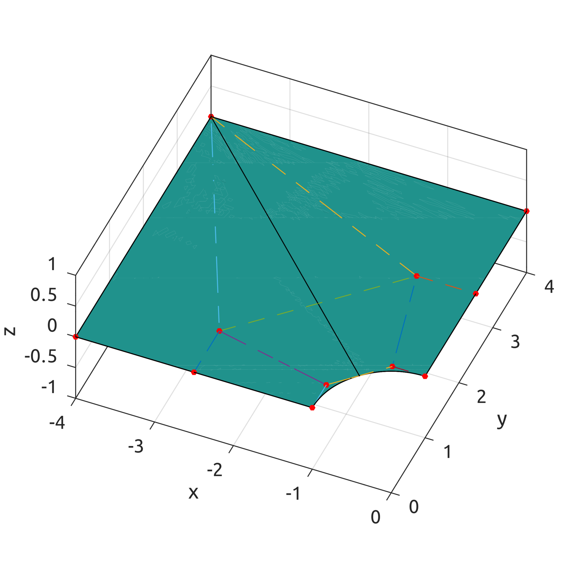
Now with the computeNURBSSurfPoint, using homogeneous coords, we can draw some interesting surfaces. Scripts are included to draw a plate with a hole:
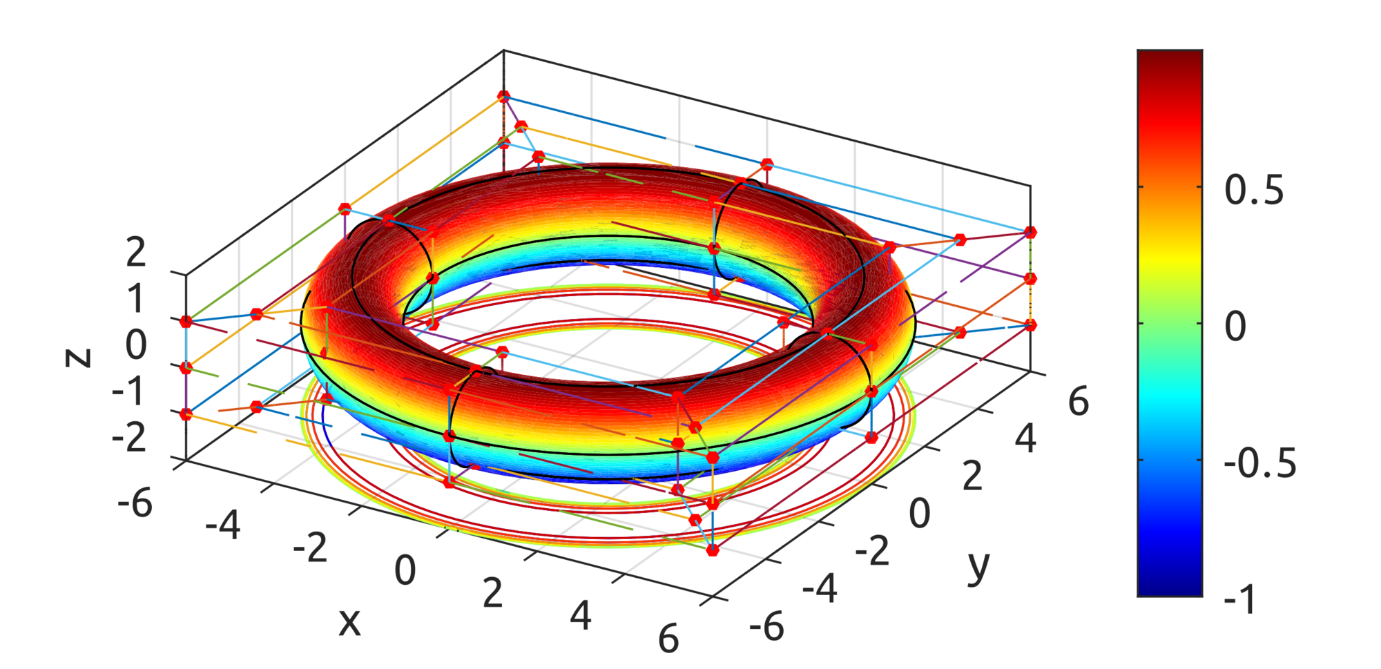
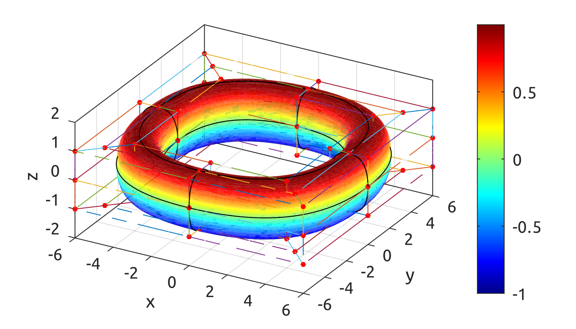
and one is provided to draw a toroid:

TypeScript Implementation

The same implementation is provided for TypeScript, so you can experiment with the browser. With the NurbsCurve you can compute NURBS basis functions:

Saturday, June 26, 2021

Isogeometric Analysis: B-spline Curves and Surfaces in Octave and TypeScript

In the previous blog post here I implemented Bézier curves. There are other important structures that are used in computer graphics and I'd need those structures to define a domain and a solution in IGA for my implementation here: https://github.com/carlonluca/isogeometric-analysis.

Bézier curves are great, but the polynomials needed to describe some curves may need a high degree to satisfy multiple constraints. To overcome this problem, some structures were designed to use piecewise-polynomials instead. Examples in this case are NURBS and B-splines.

B-spline Curves

B-splines are curves that are described using piecewise-polynomials with minimal support. The parametric domain is split into multiple ranges by using a vector. The general definition of a B-spline curve is:

$$\boldsymbol{C}\left(\xi\right)=\sum_{i=0}^{n}N_{i}^{p}\left(\xi\right)\boldsymbol{P}_{i},\;a\leq\xi\leq b$$
where $\boldsymbol{P}_{i}$'s are the control points of the curve and the functions $N_{i}^{p}\left(\xi\right)$ are basis functions defined as:

$$N_{i}^{0}\left(\xi\right)=\left\{ \begin{array}{ll}1, & \xi_{i}\leq\xi<\xi_{i+1}\\0,&\text{otherwise}\end{array}\right.,a\leq\xi\leq b$$ $$N_{i}^{p}\left(\xi\right)=\frac{\xi-\xi_{i}}{\xi_{i+p}-\xi_{i}}\cdot N_{i}^{p-1}\left(\xi\right)+\frac{\xi_{i+p+1}-\xi}{\xi_{i+p+1}-\xi_{i+1}}\cdot N_{i+1}^{p-1}\left(\xi\right),a\leq\xi\leq b$$
The values $\xi_{i}$ are elements of the aforementioned knot vector, defined as:

$$\Xi=\left[\underset{p+1}{\underbrace{a,\ldots,a}},\xi_{p+1},\ldots,\xi_{n},\underset{p+1}{\underbrace{b,\ldots,b}}\right],\left|\Xi\right|=n+p+2$$
where $p$ is the degree of the basis functions. A knot vector in this form is said to be nonperiodic or clamped or open.

B-spline Surfaces

By using the tensor product we can obtain B-splines in spaces of higher dimension. For surfaces, given the knot vectors:

$$\Xi=\left[\underset{p+1}{\underbrace{a_{0},\ldots,a_{0}}},\xi_{p+1},\ldots,\xi_{n},\underset{p+1}{\underbrace{b_{0},\ldots,b_{0}}}\right],\left|\Xi\right|=n+p+2$$ $$H=\left[\underset{q+1}{\underbrace{a_{1},\ldots,a_{1}}},\xi_{q+1},\ldots,\xi_{m},\underset{q+1}{\underbrace{b_{1},\ldots,b_{1}}}\right],\left|H\right|=m+q+2$$
a B-spline surface can be defined as:

$$\boldsymbol{S}\left(\xi,\eta\right)=\sum_{i=0}^{n}\sum_{j=0}^{m}N_{i}^{p}\left(\xi\right)N_{j}^{q}\left(\eta\right)\boldsymbol{P}_{i,j},\;\left\{ \begin{array}{c} a_{0}\leq\xi\leq b_{0}\\ a_{1}\leq\eta\leq b_{1} \end{array}\right.$$
where $p$ and $q$ are the degrees of the polynomials. In the implementations, sometimes I preferred the matrix form of the equations:

$$\boldsymbol{C}\left(\xi\right)=\left[N_{i-p}\left(\xi\right),\ldots,N_{i}\left(\xi\right)\right]\cdot\left[\begin{array}{c} \boldsymbol{P}_{i-p}\\ \vdots\\ \boldsymbol{P}_{i} \end{array}\right],\;\xi\in\left[\xi_{i},\xi_{i+1}\right)$$
For the surfaces instead, the matrix form is: $$\boldsymbol{S}\left(\xi,\eta\right)=\left[N_{i-p}\left(\xi\right),\ldots,N_{i}\left(\xi\right)\right]\cdot\left[\begin{array}{ccc} \boldsymbol{P}_{j-q,i-p} & \cdots & \boldsymbol{P}_{j-q,i}\\ \vdots & \ddots & \vdots\\ \boldsymbol{P}_{j,i-p} & \cdots & \boldsymbol{P}_{j,i} \end{array}\right]\cdot\left[\begin{array}{c} N_{j-q}\left(\eta\right)\\ \vdots\\ N_{j}\left(\eta\right) \end{array}\right],$$ $$\xi\in\left[\xi_{i},\xi_{i+1}\right),\eta\in\left[\eta_{j},\eta_{j+1}\right)$$
These forms leverage a more performant algorithm for the computation of the basis functions, which returns the value of all nonvanishing functions for a point in the parametric space. The Octave implementation is clearly simpler as Octave has native support for matrices, the TypeScript implementation instead includes a basic Matrix2 class that offers the simplest operators.

Octave Implementation

An implementation for Octave is provided in https://github.com/carlonluca/isogeometric-analysis/tree/master/3.4. There are examples to show how to draw B-spline curves with the implementation.
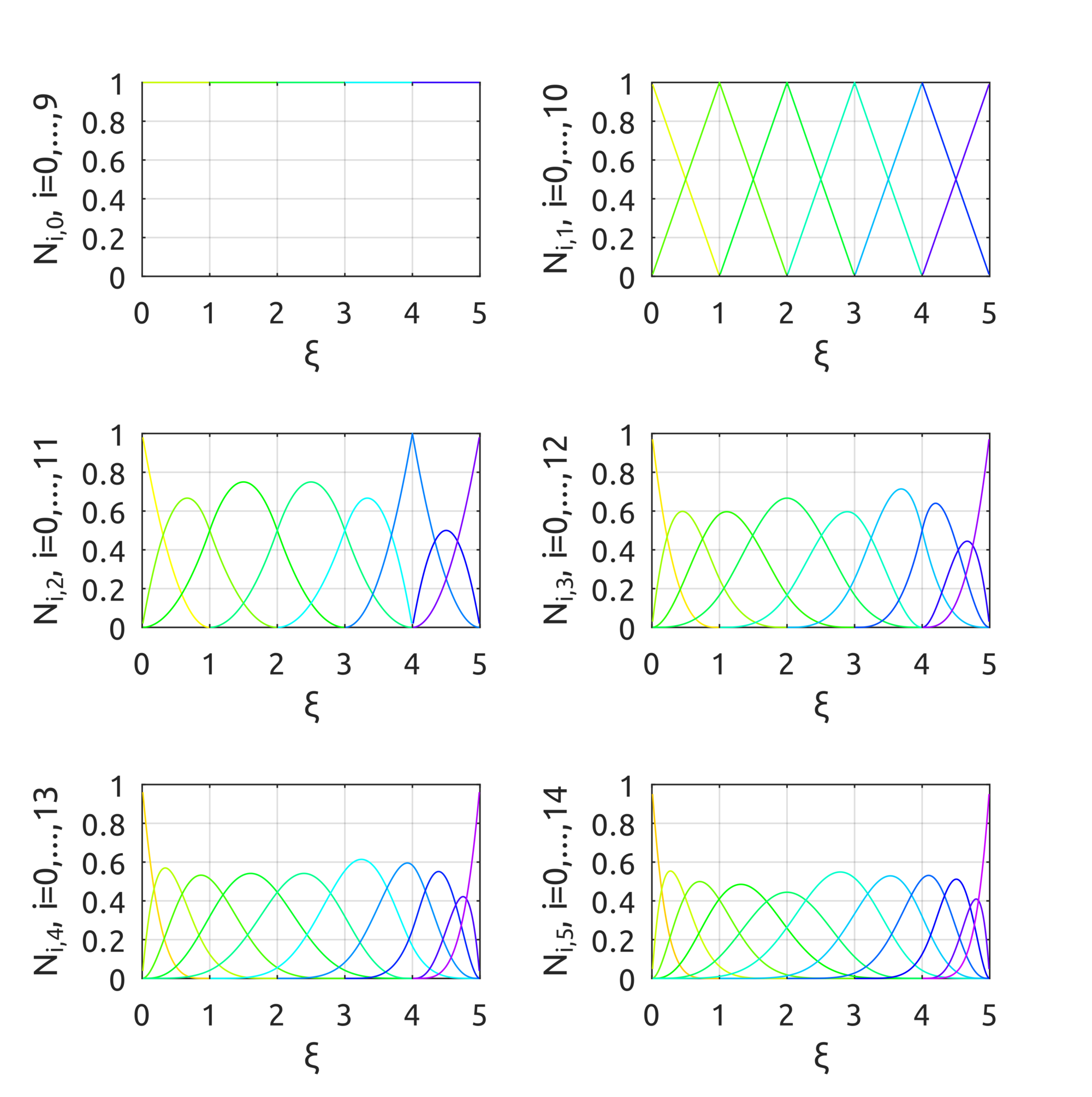
For example, the drawBsplineBasisFuns script shows the B-spline basis functions over the knot vector $\Xi=[0, 0, 0, 1, 2, 3, 4, 4, 5, 5, 5]$ using the provided implementation of the basis functions:


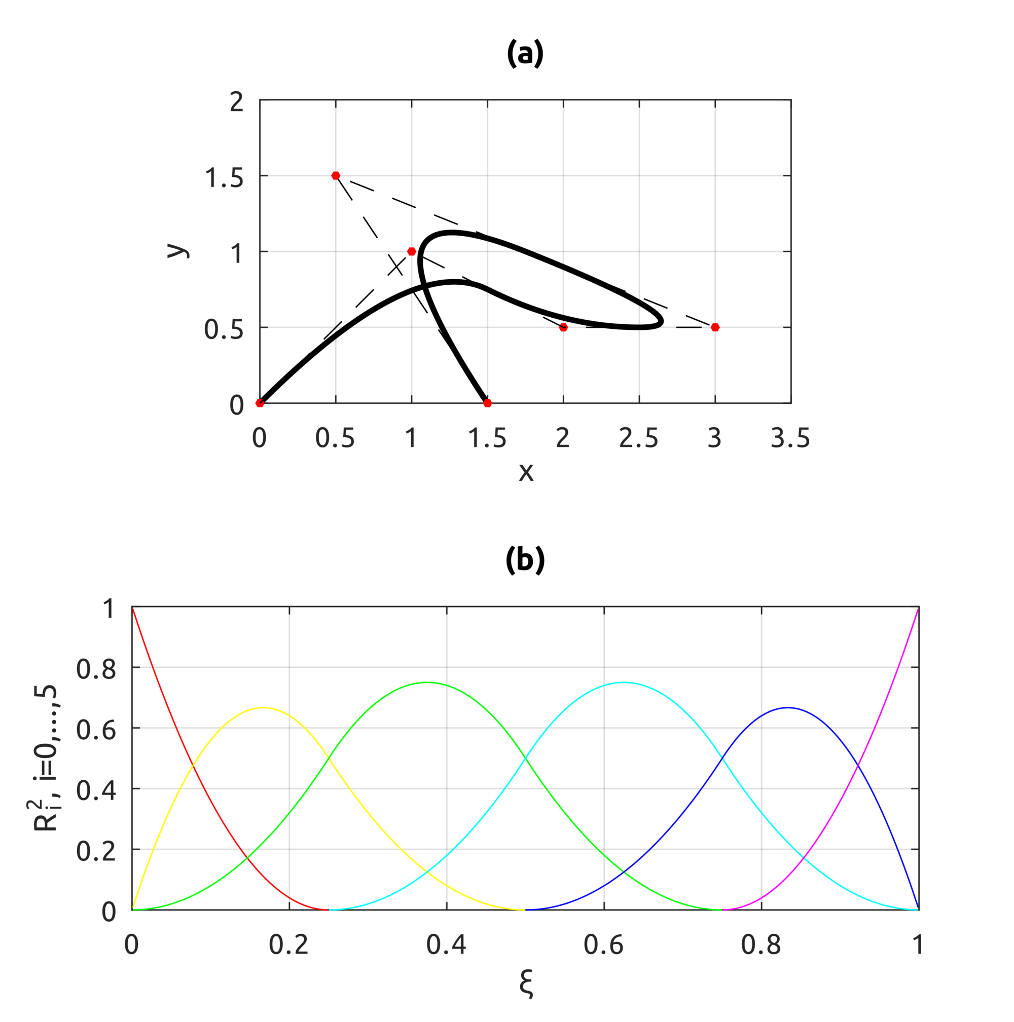
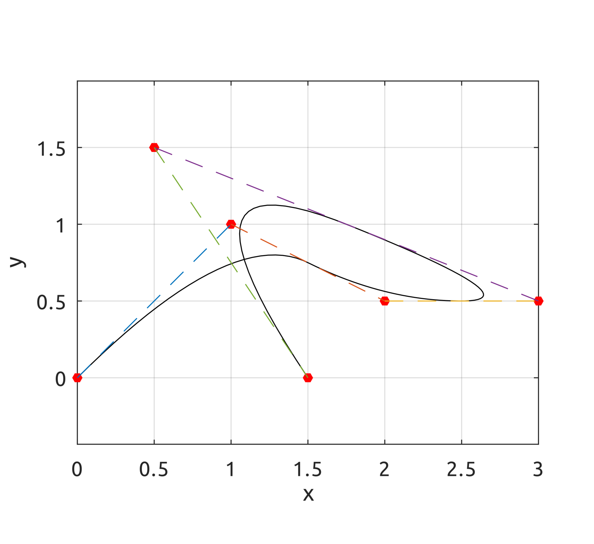
The drawBsplineCurve script draws, instead, the real curve. For example, to draw the B-spline of degree $p=2$ defined over the knot vector $\Xi=[0, 0, 0, 0.25, 0.5, 0.75, 1, 1, 1]$ with control points:

$$\boldsymbol{P}_{0}=\left(0,0,0\right),\;\boldsymbol{P}_{1}=\left(1,1,1\right),\;\boldsymbol{P}_{2}=\left(2,0.5,0\right)$$ $$\boldsymbol{P}_{3}=\left(3,0.5,0\right),\;\boldsymbol{P}_{4}=\left(0.5,1.5,0\right),\;\boldsymbol{P}_{5}=\left(1.5,0,1\right)$$

a simple call to:

drawBsplineCurve(5, 2, [
    0, 0, 0, 0.25, 0.5, 0.75, 1, 1, 1
], [
    0, 0; 1, 1; 2, 0.5; 3, 0.5; 0.5, 1.5; 1.5, 0
]);


draws:


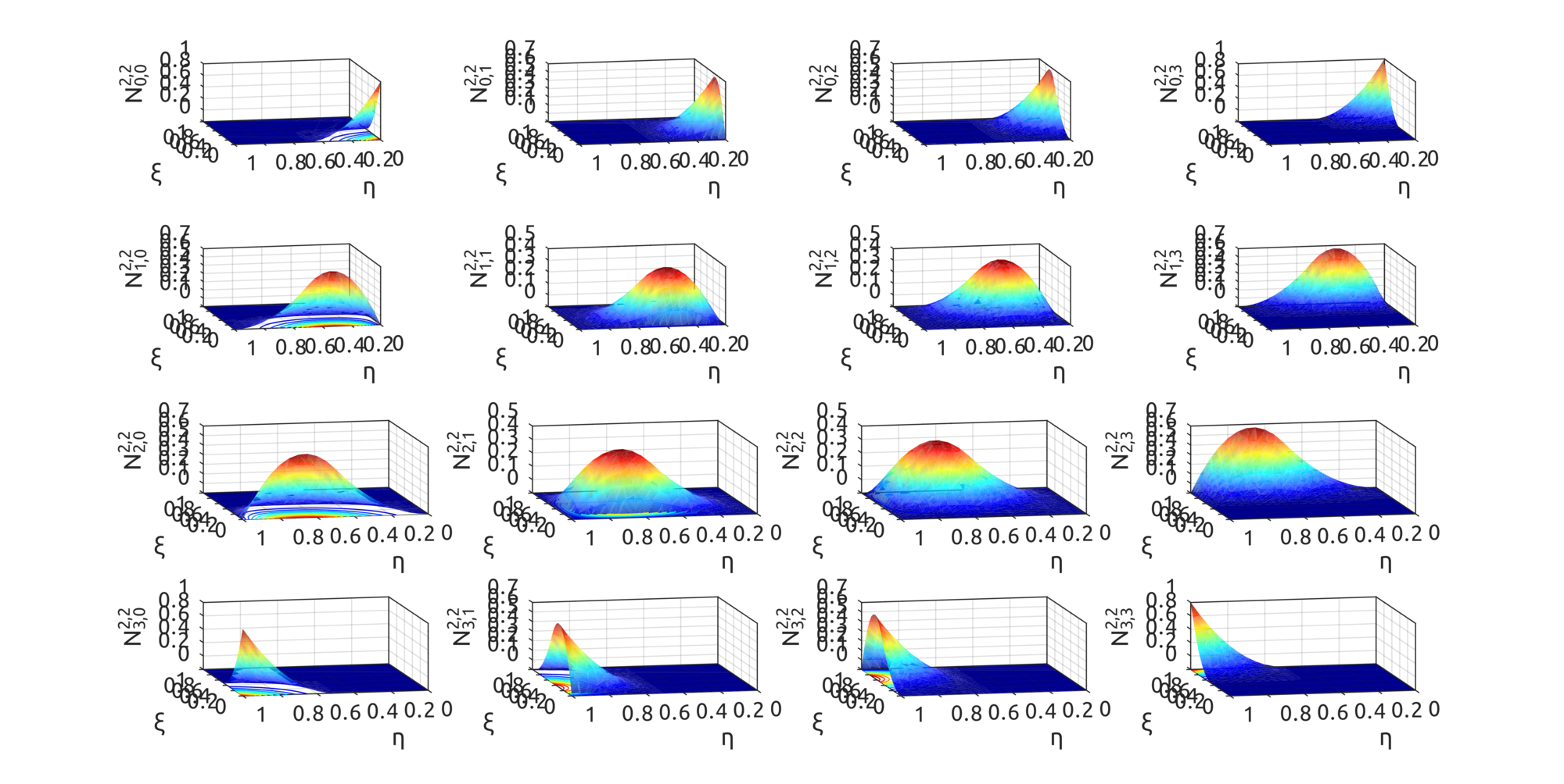
For surfaces, drawBivariateBsplineBasisFuns can be used to draw bivariate basis functions. For example:

drawBivariateBsplineBasisFuns([
    0, 0, 0, 0.5, 1, 1, 1
], 3, 2, [
    0, 0, 0, 0.5, 1, 1, 1
], 3, 2);


gives this result:

By using the defined basis functions, data defined in https://github.com/carlonluca/isogeometric-analysis/blob/master/3.4/defineBsplineRing.m can draw a shape similar to a ring:


Note that this is not yet a toroid.

TypeScript Implementation

A TypeScript implementation is also present in the repo. With a simple code like this:

Thursday, May 13, 2021

Isogeometric Analysis: Bezier Curves and Surfaces in Octave and TypeScript

While working on my sample IGA implementation here https://github.com/carlonluca/isogeometric-analysis, I found myself in need of defining and implementing the math structures used to define the domain and the solution space. This means that I had to implement various algorithms to define structures like Bezier, B-spline, NURBS and T-spline. So this is a quick intro to Bezier curves and surfaces with a couple of implementations.

Power Basis

A simple math structure to handle curves and surfaces is the power basis representation. Power basis representation uses polynomials, which are fast to compute and simple to handle.
A $n^{th}$-degree power basis curve can be defined in the parametric space as:

$$\begin{eqnarray*} \boldsymbol{C}\left(\xi\right) & = & \left(x\left(\xi\right),y\left(\xi\right),z\left(\xi\right)\right)\\ & = & \sum_{i=0}^{n}\boldsymbol{a}_{i}\xi^{i}\\ & = & \left(\left[\boldsymbol{a}_{i}\right]_{i=0}^{n}\right)^{T}\left[\xi^{i}\right]_{i=0}^{n}, \end{eqnarray*}$$


where the functions $\xi^{i}$ are the basis (or blending) functions. Using the tensor product scheme we can also define a power basis surface:

$$\begin{eqnarray*} \boldsymbol{S}\left(\xi,\eta\right) & = & \left(x\left(\xi,\eta\right),y\left(\xi,\eta\right),z\left(\xi,\eta\right)\right)\\ & = & \sum_{i=0}^{n}\sum_{j=0}^{m}\boldsymbol{a}_{i,j}\xi^{i}\eta^{j}\\ & = & \left(\left[\xi^{i}\right]_{i=0}^{n}\right)^{T}\left[\boldsymbol{a}_{i,j}\right]_{i,j=0}^{i=n,j=m}\left[\eta^{j}\right]_{j=0}^{m} \end{eqnarray*}$$


where:

$$ \left\{ \begin{array}{l} \boldsymbol{a}_{i,j}=\left(x_{i,j},y_{i,j},z_{i,j}\right)\\ b\leq\xi\leq c\\ d\leq\eta\leq e \end{array}\right.$$


Bezier

Bezier curves do not increase the space of curves representable by the power basis form, but introduce the concept of control point. Control points convey a clear geometrical meaning, which is very useful during the design process. So, a $n^{th}$-degree Bezier curve is defined as:

$$\boldsymbol{C}\left(\xi\right)=\sum_{i=0}^{n}B_{i}^{n}\left(\xi\right)\boldsymbol{P}_{i},\;a\leq\xi\leq b$$


where $\boldsymbol{P}_{i}$ represents the $i^{th}$ control point and:

$$B_{i}^{n}\left(\xi\right)=\frac{n!\cdot\xi^{i}\left(1-\xi\right)^{n-i}}{i!\cdot\left(n-i\right)!}$$

is the $i^{th}$ basis function (also known as Bernstein polynomial). With the tensor product scheme, we can also define a Bezier surface with:

$$\boldsymbol{S}\left(\xi,\eta\right)=\sum_{i=0}^{n}\sum_{j=0}^{m}B_{i}^{n}\left(\xi\right)B_{j}^{m}\left(\eta\right)\boldsymbol{P}_{i,j},\;\left\{ \begin{array}{l} a\leq\xi\leq b\\ c\leq\eta\leq d \end{array}\right.$$

Octave Implementation

In the repo https://github.com/carlonluca/isogeometric-analysis, you can find a basic implementation of Bezier curves and surfaces written for Octave (and Matlab) in: https://github.com/carlonluca/isogeometric-analysis/tree/master/3.3. The implementation is tested with a few examples. For example, given these control points:

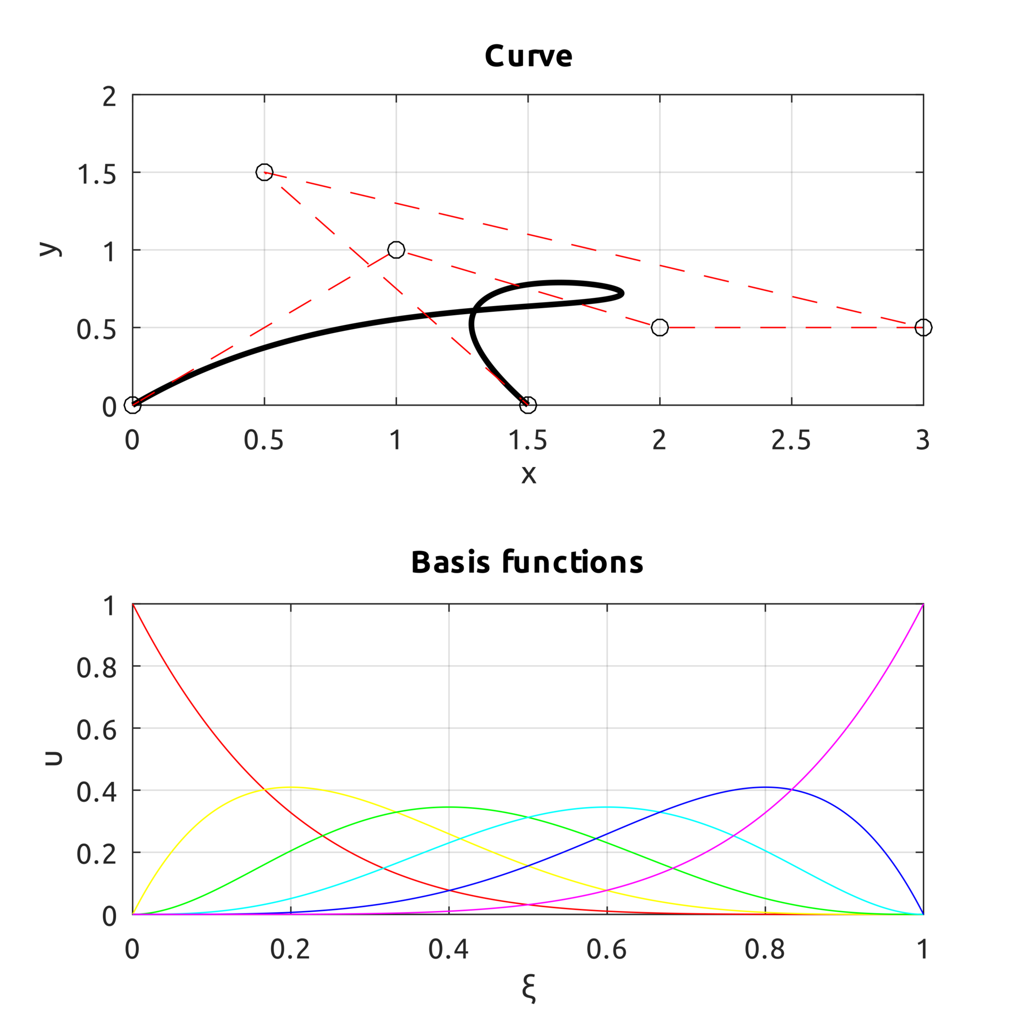
$$\boldsymbol{P}_{0}=\left(0,0\right),\;\boldsymbol{P}_{1}=\left(1,1\right),\;\boldsymbol{P}_{2}=\left(2,0.5\right)$$ $$\boldsymbol{P}_{3}=\left(3,0.5\right),\;\boldsymbol{P}_{4}=\left(0.5,1.5\right),\;\boldsymbol{P}_{5}=\left(1.5,0\right)$$


we can get to this result by using the computeBezier.m script:


We can also define the curve in the 3D space. For example these control points:

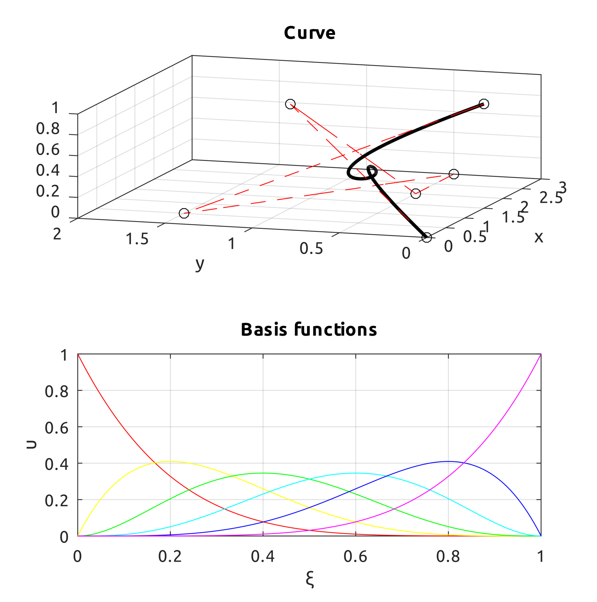
$$\boldsymbol{P}_{0}=\left(0,0,0\right),\;\boldsymbol{P}_{1}=\left(1,1,1\right),\;\boldsymbol{P}_{2}=\left(2,0.5,0\right)$$ $$\boldsymbol{P}_{3}=\left(3,0.5,0\right),\;\boldsymbol{P}_{4}=\left(0.5,1.5,0\right),\;\boldsymbol{P}_{5}=\left(1.5,0,1\right)$$

lead to this result:


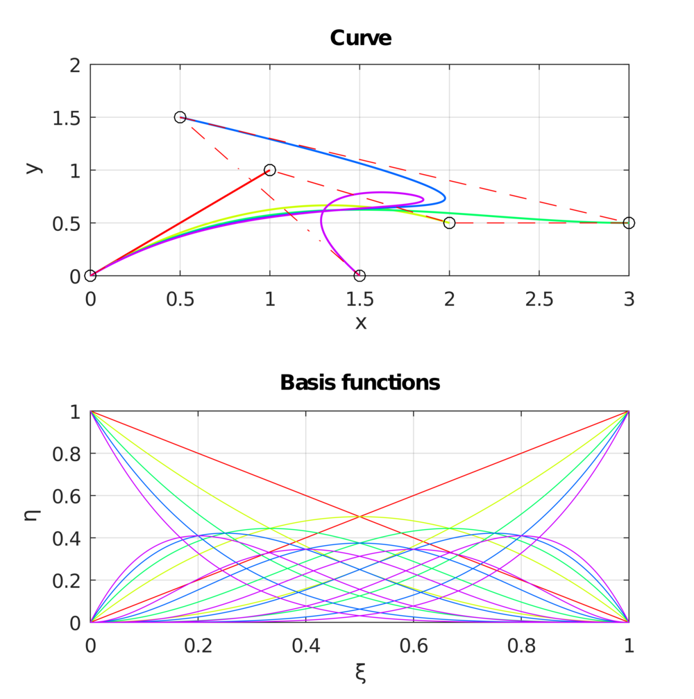
It may also be interesting to see what happens to a curve when a new control point is added to the previous one:

Another example is provided for Bezier surfaces. From these control points:

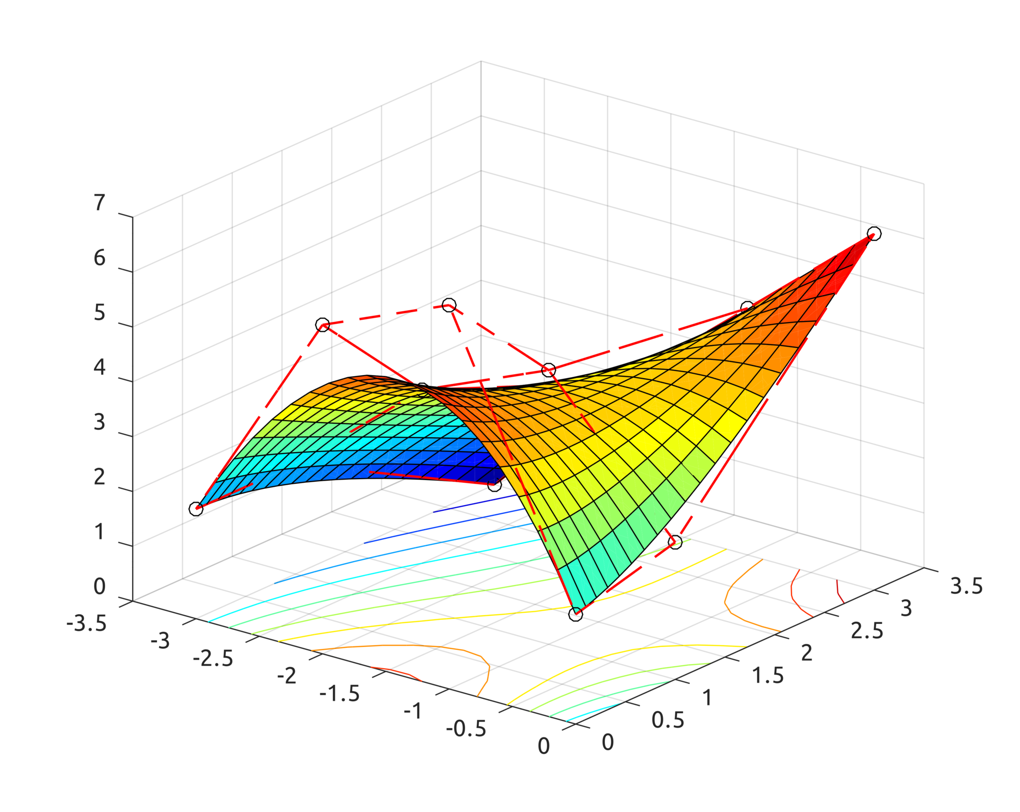
$$\boldsymbol{P}_{0}=\left(-3,0,2\right),\;\boldsymbol{P}_{1}=\left(-2,0,6\right),\;\boldsymbol{P}_{2}=\left(-1,0,7\right),\boldsymbol{P}_{3}=\left(0,0,2\right)$$ $$\boldsymbol{P}_{4}=\left(-3,1,2\right),\;\boldsymbol{P}_{5}=\left(-2,1,4\right),\;\boldsymbol{P}_{6}=\left(-1,1,5\right),\;\boldsymbol{P}_{7}=\left(0,1,2.5\right)$$ $$\boldsymbol{P}_{8}=\left(-3,3,0\right),\;\boldsymbol{P}_{9}=\left(-2,3,2.5\right),\;\boldsymbol{P}_{10}=\left(-1,3,4.5\right),\;\boldsymbol{P}_{11}=\left(0,3,6.5\right)$$


this is what the algorithms produce:

Typescript Implementation

What about a browser implemenation? The above algorithms can clearly be implemented in a browser, so this is an attempt written in TypeScript: https://github.com/carlonluca/isogeometric-analysis/tree/master/ts/src/bezier. The BezierCurve object can be used to draw a plot of the first examples: